CytoSpec - an APPLICATION FOR HYPERSPECTRAL IMAGING |
|||||||


|
|||||||
|
|
|
||||||
|
|
|||||||
Menu Bar 'Tools' |
|||||||
|
|||||||
Display Spectra |
|||||||
|
|||||||

 Load
Load 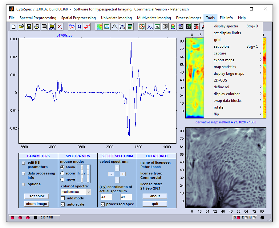
|
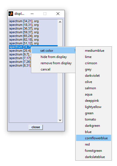
Activate the context menu by selecting one or more spectra and a right mouse click. |

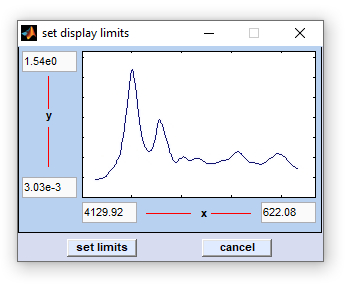
Set Display Limits
The function 'set display limits' permits manually entering display limits of the spectral panel. The dialog box is available via the
option 'set display limits' from the 'Tools' menu bar o by pressing the respective button from CytoSpec's button line.
|
|
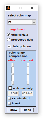
Select and Adapt Colormaps
Select and adapt colormaps of pseudo-color images.
|
select colormap: allows selection of one of the following colormaps: jet, hsv, hot, cool, bone, winter, summer, autumn, copper, prism, flag, lines, colorcube, i-jet, i-hsv, i-hot, ann, blue-black, red-black, green-black, yellow-black, white-black, cyan-black, magenta-black, blue-white, red-white, green-white, yellow-white, black-white, cyan-white, magenta-white (the latter are useful when creating |
Illustration of the effect of the check box 'interpolation':
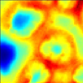
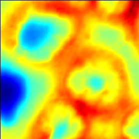
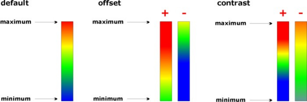
Illustration of the effects of changing the sliders 'offset' and 'contrast':
(example of the colormap 'jet')
The colormap ann (artificial neural network): This colormap is particularly useful to generate maps on the basis of classification methods producing crisp class membership values, such as:
The colormap ann can be individually modified by editing a simple text file 'color.txt'. This file is located in CytoSpec's root directory, usually in C:\program files\CytoSpec\CytoSpec (pre-2.00.05 versions of CytoSpec), or C:\Users\Public\Documents\Matlab (v. 2.00.05 and later) and is read by CytoSpec upon initialization. When editing this file, please use only color names given atHCA imaging - images re-assembled on the basis of hierarchical clustering
An example of the content of the file color.txt is given here:
The settings of the colormap ann define also the following color sequences:
- color options of the 'set color' function available from the context menu of the
display spectra function.
- selectable colors available from the listbox 'color of spectra' of the
display options window.
- the color sequence is furthermore used to display cluster average spectra of the functions
KMC , FCM and
HCA imaging (button 'spectra' → button 'plot averages
').
Grid On/Off
This option is available from the 'Tools' menu bar and has effect on the spectral plot window, only. The grid ON/OFF function may be
useful when the spectral window is exported via the Capture →
Spectral Plot function.
Capture
The function capturing false color images is available from the 'capture' option of the 'Tools' menu bar. One can either save
the image to a local / network drive hard drive (as bitmaps, map produced on the basis of original, or processed data, spectral window),
or alternatively capture the entire CytoSpec window (gui) to the clipboard.
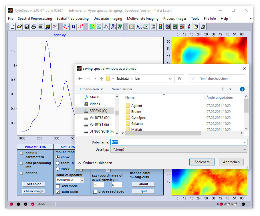
Saving images as bitmaps: Images reassembled on the basis of original spectral data (tools → capture → upper image )
and of processed spectra (tools → capture → lower image ) can be captured. When the corresponding option was selected, it
is asked to type in a path and a file name. In order to store the spectral plot you have to select the 'capture → spectral plot'
option of the 'Tools' menu bar. The option Grid ON/OFF activates
or deactivates a grid of the spectral plot (tools menu) The standard resolution used to capture the bitmaps is 300 dots per inch (dpi).
Files are stored in a standard windows bitmap (.bmp) data format.
Capturing program window: Along with storing images or spectra you may also want to take a screenshot of the program window. By
choosing the 'capture' → 'window' option of the 'Tools' menu bar and selecting the resolution (72, 150, 200,
or 300 dpi) the entire CytoSpec program window is copied to the clipboard.
Other options to export false color images: The function 'capture' is also available from so-called large maps, i.e. false color
images displayed in the true aspect ratio, see functions
display large maps and options 'composite image' of
the FCM, VCA and n-findr imaging functions (for details see the description of the respective function in
Multivariate Imaging).
Capturing false color images, spectra, or the complete gui
Capturing program window: Along with storing images or spectra you may also want to take a screenshot of the program window. By choosing the 'capture' → 'window' option of the 'Tools' menu bar and selecting the resolution (72, 150, 200, or 300 dpi) the entire CytoSpec program window is copied to the clipboard.
Other options to export false color images: The function 'capture' is also available from so-called large maps, i.e. false color images displayed in the true aspect ratio, see functions
Export Maps (Export Image Plane Data)
This function exports image plane data that are used to plot the given false-color image. Image plane data are extracted from the
hyperspectral data cubes. Such data form 2D matrices of the size [xdim, ydim] with xdim and ydim denoting the number of pixels in x-
and y-direction, respectively. Data are stored in a standard ASCII text file format. Select the option 'export maps → upper
plot (or lower plot)' from the 'Tools' menu bar to export the image data. A standard windows dialog box will appear.
Indicate then the path and the file name to be stored.
Image data will be stored in the following format (example of an image consisting of M x N pixel spectra, [xdim x ydim]):
|
1 2 3 4 5 6 7 8 9 10 . M |
1 0.2 0.4 0.5 0.7 0.8 0.9 0.7 0.4 0.2 0.6 . 0.6 |
2 0.1 0.7 0.4 0.2 0.4 0.9 0.7 0.4 0.8 0.2 . 0.5 |
3 0.2 0.4 0.5 0.7 0.8 0.9 0.7 0.4 0.2 0.6 . 0.3 |
4 0.1 0.7 0.4 0.2 0.4 0.9 0.7 0.4 0.8 0.2 . 0.1 |
. . . . . . . . . . . . . |
N 0.1 0.7 0.4 0.2 0.4 0.9 0.7 0.4 0.8 0.2 . 0.9 |
The ASCII files are now available for import by to other programs such as Microsoft Excel, Origin or Matlab. Please note that the standard extension of the ASCII image data files will be '*.dat'.
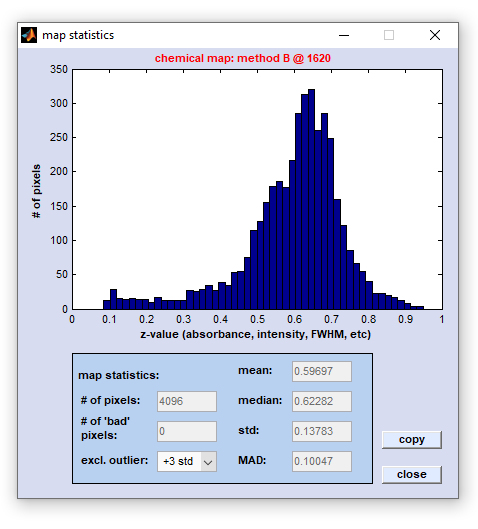
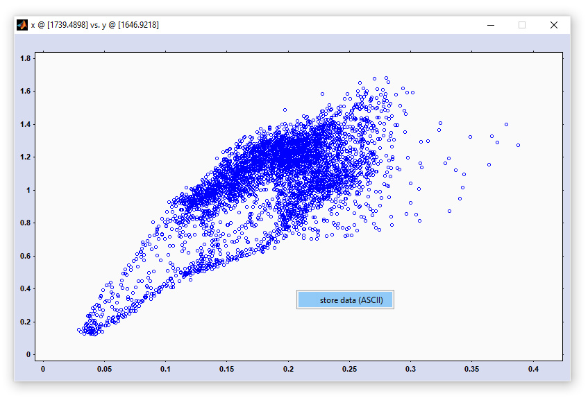
Image Statistics: Construct Histograms from Image Data
The function 'image statistics' can be used to construct histograms displaying the frequency distribution of the actual image
data (z-data) that compose the given univariate (i.e. chemical) or multivariate false-color image. Examples of univariate image
parameters are intensity values, intensity ratios, frequency positions, or half-widths of spectral bands. In cases where the function
'image statistics' was applied to multivariate images, histograms will illustrate the frequency distribution of cluster membership
values, ANN output activations, spectral distances, score values, etc. The option 'image statistics' is available from the 'Tools'
menu bar, or the context menu of a given false color image. The frequency distribution of image data can be obtained either from z-data
obtained from from original spectral data (data block #1, top right panel), or any type of processed data (bottom right panel).
|
|
Two-Dimensional Correlation Spectroscopy (2D-COS)
Two-dimensional correlation spectroscopy (2D-COS), or two-dimensional correlation analysis is known as a set of mathematical techniques
useful to study changes in dynamic spectra. Dynamic spectra are often represented by spectra series obtained from a sample that was
subjected to an external perturbation. The implementation of 2D-COS in the CytoSpec software aims to enable the analysis of spatially
resolved image (HSI) data. For this purpose a variety of methods and procedures are available, which are explained in detail in this
section of the online help. Application examples of the 2D-COS technique can be found in two scientific publications, see links at the
end of this section ('Reference to the literature').
The 2D-COS analysis technique has been initially developed by
Isao Noda in the 1980s.
Related web links:
Two-dimensional correlation
analysis (Wikipedia)
Mat2dcorr - A Matlab Toolbox for 2D-COS. This Wiki provides a
detailled description of the free 2D-COS toolbox for Matlab and allows downloding the corresponding source code. Note that a modified
version of the toolbox' source code has been used to compile CytoSpec's 2D-COS function.
Main concepts of 2D correlation spectroscopy: Basic principles of generalized 2D correlation spectroscopy are outlined in the following
publication series:
I. Noda. Two-Dimensional Infrared
(2D IR) Spectroscopy: Theory and Applications,
1990 Appl. Spectrosc. 44(4): 550-561
I. Noda. Generalized Two-
Dimensional Correlation Method Applicable to Infrared, Raman, and other Types of Spectroscopy,
1993 Appl.
Spectrosc. 47(9): 1329-1336
I. Noda. Determination of
Two-Dimensional Correlation Spectra Using the Hilbert Transform,
2000 Appl. Spectrosc. 54(7): 994-999
To start a 2D-COS analysis select '2D-COS' from the 'Tools' menu bar. This will open two different figures:
- A figure entitled '2D correlation analysis ... ' which shows the 2D correlation spectrum and mean spectra obtained from the
x- and y-spectra data
- The '2D control' figure, see description and screenshots below
Two-Dimensional Correlation Spectroscopy (2D-COS) - the 2D correlation spectrum window
1990 Appl. Spectrosc. 44(4): 550-561
1993 Appl. Spectrosc. 47(9): 1329-1336
2000 Appl. Spectrosc. 54(7): 994-999
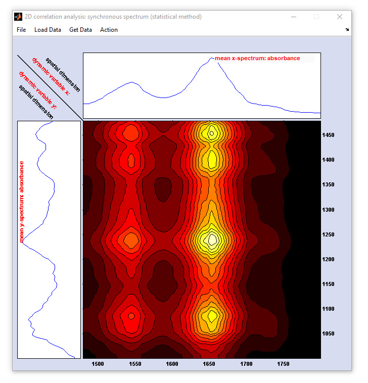
Two-dimensional correlation spectroscopy (2D-COS): screenshot of the figure for displaying the 2D correlation spectra
Loading / Getting Data for 2D-COS
Option 1.)
This options obtains x, or y-data directly from the CytoSpec workspace. Select 'Get Data' → 'Get x-data' → 'from original/ preprocessed /derivative / deconvolution data' to get the x-data. To obtain the respective y-data select 'Get Data' → 'y-data' → 'etc.'. The 'Get Data' option is available from the menu bar of the window entitled '2D correlation analysis ... ' (see window above).
Note that option 1 does not allow performing heterospectral 2D correlation analysis.
Option 2.)
Load data in the Matlab imaging format: Select 'Load Data' → 'Matlab imaging format' → 'x-data' from the menu bar of the 2D-COS window to load x-data in the Matlab imaging data format. Select 'Load Data' → 'Matlab imaging format' → 'y-data' to load the respective y-data in the Matlab imaging data format. Matlab imaging data files may contain up to four different types of hyperspectral imaging data cubes: original (unprocessed data), pre-processed, derivative and so-called deconvolution data cubes (the latter 3 types of data must be derived from the original spectral data). For a detailed description of the Matlab imaging data format see http://www.cytospec.com/file.php#FileSaveMatlab
Option 3.)
Load data in the Matlab trace format: Select 'Load Data' → 'Matlab trace format' → 'x-data' to load x-data in the Matlab trace data format. Select 'Load Data' → 'Matlab trace format' → 'y-data' to load the respective y-data in the Matlab trace data format.
For a description of the Matlab trace format see the section below.
Format of the example file 'linescandata.mat' (Matlab trace format)
Matlab trace format files contain spectra series in a 2D data format where the first dimension is the spectral dimension and the second dimension represents the perturbing variable, i.e. time, pressure, temperature, spatial dimension, etc.
Matlab trace files contain a structure array with the following fields:
- spc - this field contains the spectral data, a 2D array of double precision floating point values (float32). Columns indicate individual spectra of absorbance, intensity, transmittance, etc. values. The column length indicates the number of data points per spectrum. The number of columns is equal to the number of spectra of the spectra series.
- wav - A vector of float32 values, the 'wavenumber' vector, or more general the vector of y-values (frequencies, wavenumbers, Raman shifts or alternative variables). The length of 'wav' must equal the number of data points per spectrum, i.e. size(wav,1) == size(spec,1). Equidistancy of the 'wav' vector is not a requirement.
- tos - A character vector of variable length which indicates the type of spectra. Examples: 'Transmission', 'Fluorescence', 'Raman', etc.
- war - A vector of float32 values, which denote the perturbing variable of the experiment: temperature, time, voltage. The length of 'war' must be equal to size(spc,2)
- vst - A character vector of variable length indicating the type of the perturbing variable. Examples of vst: 'Temperature', 'Time', 'Voltage', or 'Spatial variable'
Options of the 2D-COS interactive user dialog box
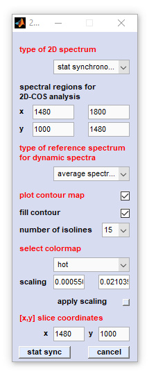
|
type of 2D spectrum: defines the type of the 2D-COS analysis, for details see below |
Options of the popupmenu 'type of 2D spectrum'
- Pearson scaling: the synchronous 2D spectrum with Pearson, or unit variance scaling. Pearson scaling is also used in statistical total correlation spectroscopy [STOCSY] and statistical heterospectroscopy [SHY])
- Pareto scale 0.75: the synchronous 2D spectrum with Pareto scaling. The parameter α equals 0.75
- Pareto scale 0.50: the synchronous 2D spectrum with Pareto scaling. The parameter α equals 0.50 (Pareto scaling in the strict sense)
- Pareto scale 0.25: the synchronous 2D spectrum with Pareto scaling. The parameter α equals 0.25
- stat synchronous: the classical (statistical) synchronous 2D (covariance) spectrum
- stat asynchronous: the classical (statistical) asynchronous 2D spectrum
- disrelation: allows to calculate the absolute of the 2D disrelation spectrum
- fft synchronous: alternative implementation to obtain the synchronous 2D correlation spectrum by means of the fast Fourier-transformation approach
- fft asynchronous: alternative implementation to obtain the asynchronous 2D correlation spectrum by means of the fast Fourier-transformation approach
Reference to the literature:
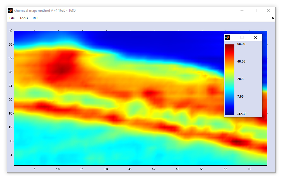
Display Large Maps
The function 'display large maps' is available from the 'Tools' menu bar but also from the context menus of
hyperspectral maps (click by the right mouse button). When this option is chosen, a new window will appear showing the maps in the true
spatial aspect ratio.
The following information can be obtained from the 'images in the true aspect ratio':
1. the pixel position of the cursor,
2. (x,y) spatial position of the cursor (obtained from the parameters SZX and
SZY)
3. the z-value (absorbance, transmittance, Raman intensity etc.) found at the current cursor location is given.
Further options:
1. the map can be stored as a bitmap by selecting 'capture to bitmap' ('Tools' menu bar).
2. a colormap is available by selecting 'display colorbar' ('Tools' menu bar).
3. the window can be deleted (chose 'exit' from the 'File' menu bar).
4. one can define Regions of Interest (ROI)
5. individual pixel spectra can be replaced by an average of their neighbor spectra, see 'replace spectra' of the
'Tools' menu bar
2. (x,y) spatial position of the cursor (obtained from the parameters
3. the z-value (absorbance, transmittance, Raman intensity etc.) found at the current cursor location is given.
2. a colormap is available by selecting 'display colorbar' ('Tools' menu bar).
3. the window can be deleted (chose 'exit' from the 'File' menu bar).
4. one can define
5. individual pixel spectra can be replaced by an average of their neighbor spectra, see 'replace spectra' of the 'Tools' menu bar
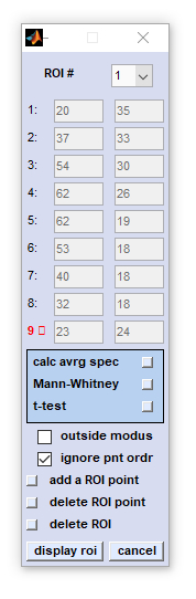
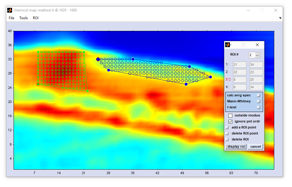
Define Region of Interest (ROI)
The function define region of interest (ROI) is available from the 'Tools' menu bar or from the context menus of false
color images of the main window (right mouse button click). When this option is chosen, a new window
Large Map will appear that shows pseudo-color images in the true spatial aspect ratio. Furthermore,
an additional interactive dialog box 'define ROI' pops up which permits definition of up to three different ROIs in an image.
|
listbox ROI #: Allows defining up to three different regions of interest. Switching between settings of these ROIs is possible by
selecting the appropriate ROI index number from this listbox
edit fields 1-15: Selection of ROI boundary coordinates can be done by clicking into image - mouse pointer coordinates will be transferred automatically. calc avrg spec (calculate average spectra): permits to calculate, display and store ROI mean spectra. This function works in exactly the same way as the option 'spectra' contained in the cluster imaging functions Mann-Whitney test: A planned feature to identify discriminating spectral features between spectra of ROI #1 and ROI#2. Not implemented yet (CytoSpec v. 2.00.07). t-test: A planned feature to identify discriminating spectral features between spectra of ROI #1 and ROI#2. Not implemented yet (CytoSpec v. 2.00.07). checkbox outside mode: this option permits switching between in- and outside modes of the ROI definition procedure. In the 'inside modus' a ROI is the defined as the region that is enclosed by the boundary. Converseyl, 'outside modus' refers to a situation where ROIs are defined as regions outside the boundary. checkbox ignore pnt ordr (ignore point order): ROI boundaries are drawn by ignoring the order of boundary points (default), or according to the order of boundary points. add ROI point: allows defining an additional ROI boundary point. The maximum number of ROI point equals 21. delete ROI point: the actual ROI point is deleted. Points can only deleted if the number of ROI points is larger than 4. delete ROI: all ROI point definitions made so far are deleted display ROI draws a region of interest cancel the routine is aborted |
Options of the menu bar 'ROI':
define ROI: This will open the dialog box 'define ROIs<(' (see above for details)
add ROI point: allows defining an additional ROI boundary point. The maximum number of ROI point equals 21.
del ROI point: the actual ROI point is deleted. Points can only deleted if the number of ROI points is larger than 4.
remove spectra in ROI: This function can be used to exclude spectra of a given ROI with the index X from the hyperspectral map. All spectra but the ROI spectra are copied from the data block of original spectra into the block of preprocessed data (existing preprocessed data may be overwritten without warning). In this way only spectral data from outside areas are transferred; pixels from ROI areas are replaced by NaN values (NaN: Not a Number). Consequently, the function 'apply ROI → preproc data → ROI #X' works in a similar way like a manual
Options of the menu bar 'Tools':
Capture to bitmap': allows storing the false color images in a *.bmp image format (including ROIs if present)
Replace spectra: this function is useful to replace individual spectra by average spectra from neighbor pixels. Requires always a predefined datablock of preprocessed spectra. Original data are not modified by this function. To replace spectra by average spectra from neighbor pixels chose 'replace spectra → on' and click onto the [x,y] coordinate with the spectrum to be corrected. More than just one spectrum can be replaced when working in replace spectra mode. In case that two, or more neighboring spectra are to be replaced it might be useful to repeatedly replace the spectra. In this way spectra with unwanted spectral features can be 'diluted' step by step. To leave the mode 'replace spectra' select the option 'replace spectra → off'.
Display colorbar: displays a colorbar of the active false-color display
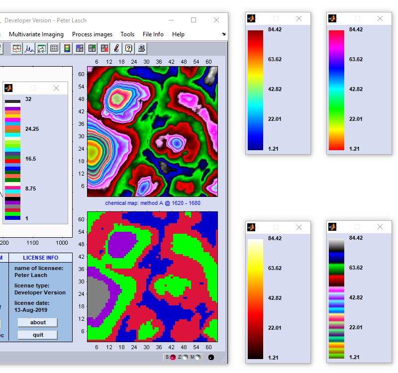
Display Colorbar
This function is available from the 'Tools' menu bar and displays a labeled colorbar of the active false color display. Note that
the colormap can be individually set by the help of the function set color
which is available from the 'tools' menu bar, or the button 'set color' (bottom left) of CytoSpec's main gui. Colorbars can
be obtained for all types of false color images, including large images
displaying false color images in their true aspect ratio, composite
images and images produced on the basis of crisp class membership values such as
HCA maps - images re-assembled on the basis of hierarchical clustering
KMC maps - images re-assembled on the basis of k-means clustering
Synthon maps - images re-assembling on the basis of Synthon's NeuroDeveloper™
neural network software
ANN maps - images re-assembled on the basis of the Stuttgart Neural Network
Simulator (SNNS)
To store the colorbar just use the context menu which offers capturing the colorbar in a bitmap image format with, or without labels.
|
Example of a colorbar of a KMC segmentation image. Note that in the example below the active colormap is of type
|
Four examples of the colorbars of the types jet (top left), hsv, colorcube and hot (clockwise direction). |
Swap Data Blocks
The swap data block function can be used to overwrite original spectral data by preprocessed data, or preprocessed data by so-called
deconvolution data, respectively (see section Internal Data Organization
to learn more about CytoSpec's concept of data blocks).
The function should be rarely employed as original data should only be modified in exceptional cases. However, the test for thickness of the
Quality Test (which can be performed exclusively on original
data) may require offset corrected spectra. As original data are lost it is highly recommended to store the data before performing the
'swap data block' function. If the block of preprocessed data is empty CytoSpec returns an error message.
To avoid overwriting of the original data as a result of typing error, CytoSpec asks for confirmation (see window below).
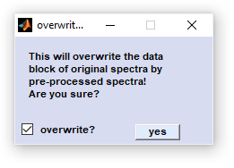
Figure swap data block.
Rotate & Flip
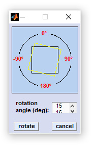
|
Data blocks AND images are manipulated such that the spatial dimensions are changed (i.e. swapping the x- and y-dimensions) while the spectral dimension remains unaffected. Rotate function can be used to rotate the data arrays by 90 degrees clockwise/counterclockwise, or by 180 degrees, respectively. The Flip function permits the flip the spectral hypercube along the x-axis ('flip horizontally'), or alternatively along the y-axis ('flip vertically') |
[
GENERAL |
FILE |
SPECTRAL PREPROCESSING |
SPATIAL PREPROCESSING |
UNIVARIATE IMAGING |
MULTIVARIATE IMAGING |
TOOLS |
FILE INFO |
GLOSSARY |
CONTACT: info@cytospec.com |
PUBLISHER DETAILS |
PRIVACY POLICY ]
Copyright (c) 2000-2026 CytoSpec. All rights reserved.
FILE INFO |
Copyright (c) 2000-2026 CytoSpec. All rights reserved.