CytoSpec - an APPLICATION FOR HYPERSPECTRAL IMAGING |
||||||||


|
||||||||
|
|
|
|||||||
|
|
||||||||
Menu Bar 'Spectral Preprocessing' |
||||||||
|
||||||||
Savitzky-Golay Derivatives |
||||||||
|
|
||||||||

 Load
Load 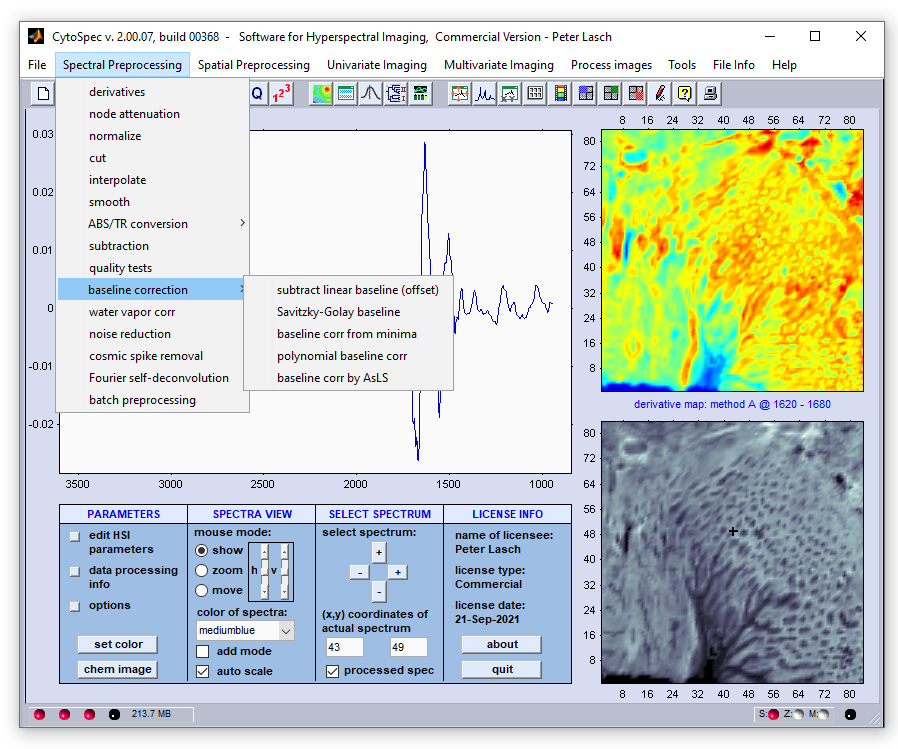
|
In vibrational spectroscopy derivative filters are popular means to enhance the apparent resolution of the spectra studied. Such filters can be routinely employed for resolving and identifying overlapping band components in complex spectral profiles. Advantages of applying derivative filters are furthermore that contributions from broad baseline artifacts are minimized which is helpful to reduce the complexity of the spectra and facilitates interpretation of spectral features. In the CytoSpec implementation derivative calculation is carried out by applying the Savitzky-Golay (SavGol) algorithm. This algorithm involves computation of n-th order derivatives while data are smoothed at the same time in order to minimize noise amplification. First or second order derivatives can be calculated including 5 to 25 smoothing points. Please note that derivatives are taken in the spectral domain, only. Details of the Savitzky-Golay algorithm used can be found in the literature:
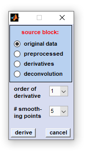
Any type of data blocks can be handled (including also derivatives). Derivative spectra are stored in a data block reserved exclusively for derivative spectra. If this block is not empty the data are overwritten without warning when obtaining derivatives again (see also Procedure: Select the source data block by clicking the appropriate radio button, then select the number of smoothing points and the order of the derivative. To start derivation click on the 'derive'' button, or hit 'cancel' to exit. |
Parameters used to obtain Savitzky-Golay derivatives are stored and are accessible through the

Node attenuation
Node attenuation has been suggested as an alternative technique for band narrowing, i.e. computational resolution enhancement
and was successfully employed in a number of vibrational spectroscopic studies. Other band narrowing, or resolution enhancement
methods are  derivative spectroscopy and
Fourier self-deconvolution. Resolution enhancement in the
spectral domain by the latter two methods proved to be an invaluable tool in the preprocessing workflow of many vibrational
spectroscopic applications, such as IR spectroscopy-based analysis of the secondary structure of proteins, or studies employing
two-dimensional correlation spectroscopy ( 2D-COS).
derivative spectroscopy and
Fourier self-deconvolution. Resolution enhancement in the
spectral domain by the latter two methods proved to be an invaluable tool in the preprocessing workflow of many vibrational
spectroscopic applications, such as IR spectroscopy-based analysis of the secondary structure of proteins, or studies employing
two-dimensional correlation spectroscopy ( 2D-COS).
The major drawbacks of derivative spectroscopy and Fourier self-deconvolution are the generation of so-called side lobes
with opposite signs adjacent to the narrowed band. Noda therefore recently suggested an alternative spectral resolution enhancement
technique, node attenuation, which was specifically designed for application in 2D-COS. This new band narrowing technique is based
on derivatives and avoids the generation of unwanted side lobes in resolution enhanced spectra.
Important: baseline correction is strongly recommended - the method of node attenuation should be
applied only to baseline corrected spectra!
|
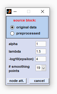
source block: please select the type of data block for node attenuation α: this parameter defines the power of the node attenuation filter: the larger α, the stronger the resolution enhancement. If the filter power α is too large, side lobe regions may be attenuated to zero, so useful information is lost for further analysis. For resolution enhancement, a value of α=1 is often adequate. λ: the peak profile factor lambda, defining the shape of the peaks. λ defines the influence of the first derivatives. If λ equals 0, peaks will have tombstone like peak profiles. Note that large values of λ may produce distorted peak shapes with a single sharp spike in the center of the peak. -log10(ε): this is the regularization constant of the node attenuation filter, required for for numerical stability. The parameter should be increased in case of distorted peak profiles. Recommended values for -log10(ε): Maximum spectral intensity *4. Note that the value indicated will be automatically multiplied by the maximum spectral intensity (default of -log10(ε): 4). # smoothing points (number of smoothing points): This parameter exerts a strong effect on the resulting resolution enhancement: large values result in smooth profiles with low resolution enhancement and vice versa. Node attenuation involves calculation of first and second derivatives by using the ( button node att. (node attenuation): starts the filter routine of node attenuation cancel: The node attenuation routine is aborted |
Node attenuation parameters are stored and are accessible through the
Reference to the literature:
Normalization
|
The CytoSpec 'normalization' function currently offers six different methods for spectra normalization:
1-norm: spectra of an HSI are normalized by dividing each spectrum by its sum of absolute intensity/absorbance values of the spectral region indicated. 2-norm: spectra are normalized by dividing each spectrum by its sum of squared intensity/absorbance values of the spectral region indicated. Maximum norm (infinity norm): spectra are normalized by dividing each spectrum by its maximum intensity/absorbance value of the spectral region indicated. Offset correction: performs are linear correction of each spectrum by subtracting its minimum intensity/absorbance value from the spectrum. In this way at least one point of the spectral region indicated equals zero. Spectra are not scaled in this mode. Standard Normal Variate (SNV): A standard normal variate is a normal variate with mean μ=0 and standard deviation σ=1. SNV normalization is achieved by dividing mean-centered spectra by their standard deviation over the spectral intensities giving the resulting spectra a unit standard deviation of one. Vector normalization: is carried out in the following way: spectra are first mean-centered by subtracting mean values of the given spectral region. Then, the spectra are scaled such, that the sum squared deviation over the indicated wavelength interval equals one. 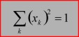
|
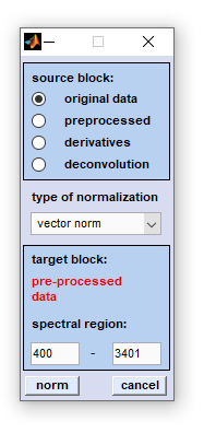
To normalize spectra of a given HSI select first the source data block by activating the appropriate radio button (see also
To start normalization click onto the 'norm' button. If you wish to cancel the operation press 'cancel'.
The normalization method and the parameters used for normalization, such as spectral range, are stored and are accessible through the
Cut Spectra
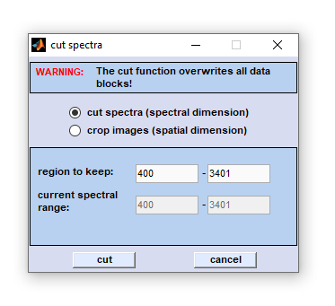
CytoSpec's 'cut' subroutines offer two different ways to cut spectral domain data, or crop image domain data of
hyperspectral data sets:
- Cutting in the spectral domain, and
- Crop images in the spatial domains.
|
Cutting in the spectral (z)- dimension can be used to narrow the frequency range of spectral data files. This may be useful to free some memory before memory-consuming calculations such as 3D Fourier self-deconvolution are carried out. Define the frequency range to be kept, then click on the 'cut' button to start the function. Pressing the button 'cancel' aborts the operation. Note that the 'cut/crop' function overwrites all existing data blocks (see also Parameters used to cut spectra are stored and are accessible through the |
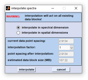
Interpolation (Spectral Domain)
CytoSpec's 'interpolation' routines offers interpolation of HSI data, either of spectra of or images:
- interpolation in the spectral domain (this function), and
- interpolation in the spatial domains
|
Interpolation in the spectral (z)- dimension changes the spacing between spectral data points. The spacing can be increased or decreased by the 'interpolation factor', which is allowed to vary between 1/32 and 32. For example, if a factor of 4 is chosen, the number of data points is increased by a factor of 4, i.e. one frequency interval is filled with (4-1) additional data points. In this case the program performs one-dimensional interpolation of the spectra. Note that the number of data points of the interpolated spectrum may become rather large when using a large interpolation factor (e.g. 32). The actual number of data points depends on the start and end frequency values and the frequency interval spanned by the original spectrum. If a factor smaller than 1 is chosen, the data point spacing is increased. For example, if a factor of 0.25 is chosen, the number of data points is decreased by a factor of 4, i.e. four frequency intervals are merged into one interval. Consequently, spectral information is lost. Interpolation can be thus useful to reduce the noise or to free some memory before memory-consuming analyses such as multivariate imaging, or 3D Fourier self-deconvolution (3D-FSD) are carried out. |
|
The 'interpolate' function overwrites all existing data blocks (see also Parameters used for interpolation are stored and are accessible through the |
|
Smoothing
Smoothing: This function is used to smooth spectra, using either the Savitzky-Golay, or the average smoothing algorithm.
Possible values for smoothing points are 5 to 25. Select the source data block as usual, choose the number of smoothing points and
click the button 'smooth' to start the operation. Smoothing has a mostly cosmetic effect on the spectra, reducing the noise
at the expense of distorting the signals.
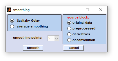
Dialog box 'smoothing spectra'
Details of the Savitzky-Golay algorithm can be found in the literature:
A. Savitzky and M. Golay. Smoothing and
Differentiation of Data by Simplified Least Squares Procedures. Anal. Chem. 1964 Vol 36(8):1627.
Parameters used for smoothing are stored and are accessible through the
File Info menu (File Info → Data processing Info →
type of data block). Parameters are also displayed in CytoSpec's report
window.
Conversion Absorbance ↔ Transmission
TR ↔ ABS conversion: This function performs the conversion from transmission spectra to absorbance spectra and vice versa.
Note: The function ABS ↔ TR acts on the complete data block of original spectra and overwrites the data block of original spectra.
Furthermore, all other types of data will be deleted.
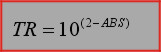
For converting absorbance spectra to transmission spectra the following formula is used:
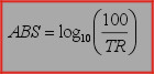
Formula, used to obtain absorbance spectra from transmission spectra:
Subtraction
Subtraction: This function permits subtraction of spectra from complete spectral data blocks. The function might be useful to
compensate for spectral contributions of supporting substrates in transmission type imaging data (example: subtraction of absorbance
spectra of thin films).
Spectral subtraction can be carried in two ways: by an internal, or an external spectrum:
- Internal spectrum - a spectrum that is contained in the actual spectral map.
- External spectrum - the spectrum can be loaded (ASCII format).
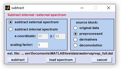
Screenshot of the dialog box 'subtraction'
Using external spectrum for subtraction: in order to use this function check the appropriate radiobutton. Load the external
ASCII spectrum (details of data format are given below). Type in the scaling factor and select the source data block. After pressing
the 'subtract' button the external spectrum will be multiplied by the scaling factor and the resulting spectrum is subsequently
subtracted from all spectra of the source data block. .
Using internal spectrum for subtraction: check the radiobutton 'use internal spectrum' and choose the (x,y) pixel positions
(coordinates) of the spectrum you wish to subtract from the map. Note that upon its initialization the 'subtract' window will
read the actual (x,y) coordinates from the main gui. Press the 'subtract' button after selecting the source data block.
Source block: Here you can choose the type of the source block for the subtraction function. Please note that deconvolution data
cannot be used as source data.
Target block: If the source data blocks are of the type original or preprocessed, the target data block will be of the type of
preprocessed data. If the source data are of the type derivative the target data block will be also of this type (existing data are
overwritten without warning, see also Internal Data Organization).
The spectral subtraction routine is always carried out on the complete 3D spectral data block.
Button load spectrum: Permits to load a double column ASCII spectrum. If the file could be successfully loaded the directory
and the file name is displayed and the button 'subtract' becomes activated.
Button subtract: Starts the subtraction routine immediately.
Button cancel: The routine is aborted.
Note: In order to be able to subtract an external spectrum one have first to produce a double column ASCII spectrum (for
details of the data format see spectra vap_cut.dat or wap_full.dat; both spectra can be found in the directory
CytoSpecRootDir/Testdata/watervap/). Upon loading the external spectrum is automatically adapted such that its data point spacing
and its frequency range fits that of the sample data:
It will be interpolated (alternative point spacing), cut (broader frequency range), and/or extrapolated (narrower range).
Extrapolation is achieved by using the closest absorbance value to fill missing data points.
Parameters employed to subtract from HSI data sets are stored and are accessible through the
File Info menu (File Info → Data processing Info →
type of data block). Parameters are also displayed in CytoSpec's report
window.
Quality Tests
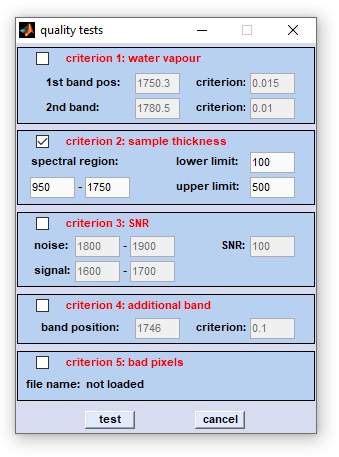
Quality Test: The function 'quality test' implemented in the CytoSpec software comprises five distinct checks for spectral
quality:
- A test for spectral contributions from atmospheric water vapor
- A check for sample thickness (uses integrated intensity values)
- The test of the spectral signal-to-noise ratio (SNR)
- A check called 'test for an additional band'
- a 'bad pixel' test (a tool to eliminate spectra from dead pixels of focal plane array (FPA) detectors
|
Data organization: the quality tests are performed exclusively on the data block of original spectra. Spectra that have passed the tests are copied without modifications to the data block of preprocessed spectra. Note that existing data of this block are overwritten without warning. If the quality test of a given spectrum is negative, the respective field in the preprocessed data block is replaced by NaN (Not a Number). In this way, spectra tested for poor quality are excluded from further evaluations and will appear in all subsequent false-color image approaches as black areas. If you wish to perform a quality test on preprocessed spectra, for example a sample thickness test after baseline correction, you have to use the To enable a test, check the appropriate checkbox and specify the quality test parameters such as absorbance thresholds. Press the button 'test' to start the quality test or hit 'cancel' if the test should be aborted. The parameters of the test for spectral quality and details of the test results can be found in the |
1. Test for water vapor:
Sharp water vapor absorption bands can be found in the spectral region between 1300 and 1800 cm⁻¹, a region where many biomaterials exhibit also strong absorption bands. It is therefore recommended to use water vapor bands above 1750 cm⁻¹ for testing. Indicate the precise positions of two water vapor bands which should be utilized for testing and define an absorption threshold criterion. If the absorption of one of the bands is higher than the specified criterion, the test result for the given spectrum will be negative, and the spectrum will be eliminated.
2. Integral absorption as a measure for sample thickness:
The absorbance, integrated over a large spectral region, can be used as a rough measure of sample thickness in transmission type measurements. As many multivariate imaging techniques such as HCA or ANN imaging require a consistent level of the SNR throughout the map, spectra with too low absorptions have to be excluded from further multivariate analysis. On the other hand you may want to eliminate also spectra showing intense signals. This could be the case where the Beer-Lambert law is not obeyed (total absorption, non-linear detector response, etc.)
In order to apply the 'sample thickness' criterion indicate the spectral region to be used for obtaining the integral. Next, define a upper and a lower threshold for the integral (edit field lower/upper limit). Check the appropriate checkbox to enable the test. A spectrum has failed the sample thickness test if an integration value is determined which is higher or lower than the defined thresholds.
3. Signal/noise ratio (SNR):
This test allows the signal-noise-ratio for individual spectra to be calculated, and to eliminate those that do not fulfill a threshold SNR ratio. Indicate the spectral regions to be used for defining the noise and signal, respectively. For biomedical samples, it is recommended to obtain the signal in the amide I region (1600 - 1700 cm⁻¹) and the noise in the region between 1800-1900 cm⁻¹. Also indicate the SNR threshold and check the checkbox for the SNR test. Spectra are rejected if the SNR is lower than the threshold.
Noise: the standard deviation in the defined spectral range:4. Test for an additional band:
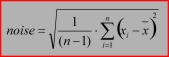
Signal: the maximum ordinate value in the defined wavenumber range<
This test is useful to exclude spectra from the data set that contain an artifact band (example: regions of a tissue section contaminated by tissue embedding medium). Indicate a typical band position (carbonyl esters of tissue freezing medium: 1746 cm⁻¹) and an absorbance threshold (edit field criterion). Spectra with a higher absorbance at this frequency will be eliminated.
5. Elimination of 'bad' pixel from FPA data:
Most of the focal plane array (FPA) detectors have so-called 'dead pixels', i.e. detector elements with zero response to IR radiation. The spectral information at these FPA elements is usually replaced by the camera software with interpolated data from pixel neighbors. If you wish to remove interpolated spectra from the data set, you have to create a simple text file, which should contain the dead pixel (x,y) positions. The text file can be loaded by activating the appropriate check box. Spectra at the given positions are then replaced by NaNs (not a number), i.e. excluded from all subsequent calculations.
Please note: Please use the function
Quality test parameters are stored and are accessible through the
Video tutorial spectral and spatial preprocessing with CytoSpec (Youtube):
(in this video, utilization of the function 'quality test (thickness test)' is exemplified after position 0:30 min)
Spectral Baseline Correction
Baseline correction: This set of functions can be used to perform correction of spectral baselines. Five different
algorithms for baseline correction are currently available:
- Subtract linear baseline (offset)
- Savitzky-Golay baseline correction
- Baseline correction from curve minima
- Polynomial baseline correction
- Baseline correction by asymmetric least squares
1. Subtract linear baseline (offset): Identical to the offset correction option of the
Normalization function. It performs are linear correction of the complete spectrum such that at least
one point of the spectral region indicated equals zero. Spectra are not scaled in this mode.
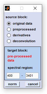
|
source block: please select a data block you wish to correct (normalize) by the linear baseline (offset) correction routine. spectral region: the spectral region, in which the baseline function is searching for a minimum y-value of the spectrum which is subtracted from the spectrum. norm: clicking on the 'norm' button corrects the baseline. cancel: closes the application. |
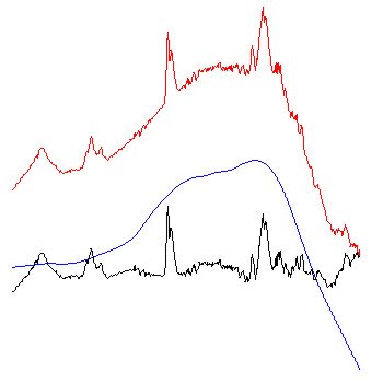
2. Savitzky-Golay baseline correction: This function can be used to automatically compensate for baseline effects, for instance as a result of scattering. As it is illustrated in the figures below, spectral baseline curves are generated by Savitzky- Golay filtering using a very high number of smoothing points (up to 999).
Baseline corrected spectra are obtained by subtracting the baselines from the original spectra.
Baseline correction can be carried out on original (absorbance/transmittance/Raman intensity) spectra and preprocessed spectra. Please note, that in the latter case existing data are overwritten without warning. Details of CytoSpec's internal data organization can be found in the respective chapter of the CytoSpec online help (
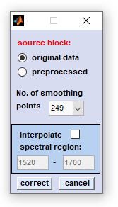
|
source block: please select a data block you wish to compensate for non-linear baseline effects. number of smoothing points: number of smoothing points used for Savitzky-Golay smoothing. interpolate spectral region: a spectral region, in which the slope of the baseline should be interpolated. To activate this feature you have to check the appropriate checkbox and to indicate the wavenumber values of the spectral region you wish to exclude from baseline calculation (in biomedical spectroscopy, this may be the amide I and II region: 1520-1700 cm⁻¹). correct: the baseline correction procedure is initiated. cancel: closes the application. |
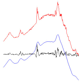
Example: The figure below exemplary illustrates how the algorithm of Savitzky-Golay baseline correction works.
red spectra: original FT-IR absorbance spectra.
blue spectra: baseline curves as obtained by integration of extensively smoothed spectra . The left part of the figure shows baselines obtained with 99 smoothing points and the right panel with 249 points (resolution in the original spectra: 8 cm⁻¹; zero-filling-factor of 4; data point spacing: 2). The example to the right demonstrates additionally the effect of the option 'interpolate region' which was used to interpolate the baseline in the amide I and II regions (1520 - 1700 cm⁻¹).
black spectra: red (original) minus blue (baseline) spectra. These spectra are stored in the data block of preprocessed spectra.
Note: due to the of Savitzky-Golay algorithm, baseline correction might be ineffective in regions close to the upper and lower wavenumber limits (UWN, LWN), particularly if a high number of smoothing points have been chosen. If the number of smoothing points is NOP and the data point spacing is DPS, the baseline correction routine will perform a linear extrapolation of the baseline in the spectral regions
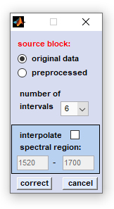
3. Baseline correction from curve minima: The function divides the spectrum in segments, or intervals in which minimum y-values (absorbance, Raman intensities) are obtained. These y-values are in the following used to generate a baseline correction curve (by shape-preserving piecewise cubic interpolation) which is then subtracted from the original spectrum.
|
source block: please select a data block you wish to compensate for non-linear baseline effects. Note that this function does not work on derivative, or deconvolution data. number of intervals: number of intervals in which the spectrum is divided. interpolate spectral region: a spectral region, in which the algorithm should not search for baseline points. If this option is activated you are able to enter the wavenumber values of this spectral region. correct: starts the baseline correction routine. cancel: the window is closed |
4. Polynomial baseline correction: This function can be used to subtract a baseline from spectra. The baseline function is a n-th order polynom, which is obtained from a set of baseline points that can be defined either automatically, or manually.
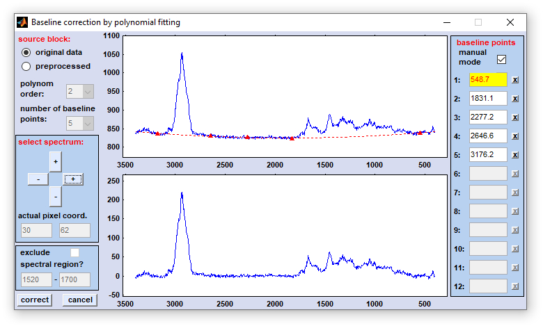
source block: please select a data block you wish to compensate for non-linear baseline effects. Note that this function does not work on derivative or deconvolution data.
polynom order: order of the polynom. Valid values are 2-10. Please try to avoid high-order polynoms.
number of baseline points: select here up 2-12 points which are used to obtain the polynomial baseline function. Note that the number of points should be larger than the order of the polynom.
select spectrum: the windows to the right display normally the original spectrum with the actual baseline function (upper panel) and the corrected spectrum in the lower panel. The spectrum is read upon initialization of the polynomial baseline function from the main window. If you wish to check the effect of baseline correction on alternative spectra you can increase/decrease the coordinates of the actual test spectrum by pressing one of the four buttons of this panel. The actual pixel spectrum coordinates are displayed in the fields 'actual pixel coord.'
interpolate spectral region: a spectral region, in which the algorithm should not search for baseline points. If this option is activated you are able to enter the wavenumber values of this spectral region.
baseline points, manual mode: allows to manually modify the position of baseline points. Check this checkbox to activate the manual definition mode. If checked one can define baseline points either by mouse-clicks in the upper central panel (shows the original spectrum and the polynomial baseline) or by entering the wavenumber/wavelength values directly in the appropriate edit fields to the right. Note that the field marked by the yellow color will be updated by the next mouse action.
NOTE: each time when the popupmenus 'polynom order' and 'number of baseline points' are modified the baseline correction function updates all baseline points by a pre-defined algorithm. Baseline points defined earlier may be lost.
x-buttons: when one of these buttons is pressed the respective baseline point is deleted (only possible in the manual mode of baseline point definition).
correct: starts the polynomial baseline correction procedure.
cancel: closes the application.
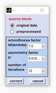
5. Baseline correction by asymmetric least squares (AsLS): A function that has been introduced with CytoSpec version 2.00.05. The AsLS function is an iterative method in which a baseline is fitted to the data.
|
source block: Please select a data block on which the baseline correction is to be performed. Note that the function 'baseline correction with asymmetric least squares (AsLS)' cannot be applied to correct derivative, or deconvolution data. smoothness factor Δ(λ): the smoothness factor defines how close the fitted baseline curve follows the spectral curve. High values of λ result in a more linear baseline and lower values lead to baselines that may resemble broad spectral bands. The parameter should be chosen such that baseline corrected spectra do not exhibit remnants of baseline features, while the spectral bands are ideally retained. asymmetry factor p: this factor determines the asymmetry by weighting the residuals based on their sign: different weights are given to baseline points having positive or negative residuals. As Raman, or absorbance spectra should not contain negative data, small values of the the asymmetry factor p should be preferably applied. number of iterations: indicates how many iterations are allowed to fit the baseline to the data. In practice convergence is often achieved after 5-10 iterations. correct: starts the baseline correction routine. cancel: closes the AsLS dialog box. |
Parameters used for spectra baseline correction are stored and are accessible through the
Reference to the literature:
Water Vapor Correction
Water vapor correction: This function is useful in IR hyperspectral imaging and permits automated subtraction of a water vapor spectrum
from measurement data such that spectral contaminations from atmospheric water vapor are minimized.
The water vapor correction routine for a single spectrum works as follows:
- A second derivative spectrum of a pure water vapor absorbance spectrum is obtained.
- Then, a second derivative spectrum is calculated from the sample spectrum.
- Depending on your selection, up to 4 separate y-values (i.e. 2nd derivative intensities) at predefined spectral positions
of water vapor bands are obtained from both derivative spectra.
- The water vapor correction factor is calculated by dividing the respective y-values obtained from the water vapor and the sample
spectrum, If more than one y-value was selected, the final water correction factor represents the average value of the ratios.
- Finally, sample data are corrected by subtracting the original water vapor spectrum multiplied by the water vapor correction factor.
Note that the correction factor is obtained from 2nd derivatves whereas subtraction is done with absorbance spectra.
- Steps 2 to 5 are carried out for all point spectra contained in the given spectral hypercube.
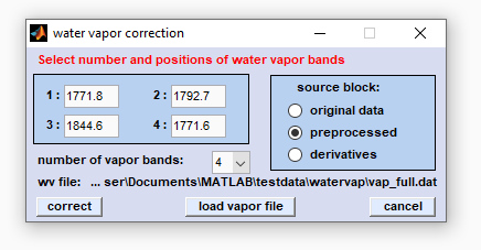
Screenshot of CytoSpec's user interface for water vapor subtraction
water vapor correction of derivative spectra: To perform water vapor correction of derivative spectra, one has to make sure
that (i) the data block of derivative data contains 2nd derivatives which (ii) are calculated by using the Savitzky-Golay algorithm
with five smoothing points. Correction will fail if these two conditions are not fulfilled.
number of vapor bands: Please choose the number of water vapor bands on which the spectral compensation for water vapor bands
should be carried out.
edit fields 1-4: Enter the correct positions (in wavenumber units) of water vapor bands. Please note that the band positions may
slightly differ from instrument to instrument (calibration) and may vary also as a function of the temperature.
Source block: Here you can choose the type of the source block for water vapor compensation.
load vapor file: Permits to load a double column ASCII water vapor spectrum. If the file could be successfully loaded the
directory and the file name are displayed and the button 'subtract' becomes activated.
correct: Starts the spectral water vapor correction routine.
cancel: The routine is aborted.
data organization (source and target data blocks): Any type of data blocks (except deconvolution data) can be handled, including
also derivative data. If the source block is of type original, or preprocessed spectra, the data are stored in the data block of
preprocessed spectra. Note that data are overwritten if this block is not empty. Water vapor corrected derivative spectra
are stored in the data block of derivative spectra, existing data are also overwritten without warning, see also
Internal Data Organization, Table II. Water vapor correction
is always carried out on the complete 3D spectral data block.
Please note: In order to spectrally compensate for water vapor one have first to produce a double column ASCII spectrum of water
vapor (for details of the data format see spectra vap_cut.dat or wap_full.dat; both spectra can be found in the following
directory: CytoSpecRootDir/Testdata/watervap/.
Upon loading the external spectrum is automatically adapted such that its data point spacing and its frequency range fits that
of the sample data:
- It will be interpolated (if the point spacing is different), cut (broader frequency range), and/or extrapolated
(narrower range).
- Extrapolation is achieved by using the closest absorbance value to fill missing data points.
In the water vapor testdata directory (CytoSpecRootDir/Testdata/watervap/) one can find a test file named 'watervap.mat'.
The first data block of this file (original data) contains the original absorbance spectra. Water vapor corrected IR absorbance
spectra are found in the second data block of preprocessed spectra. Original spectra are corrected by using the file 'vap_full.dat'.
Parameters used for water vapor correction are stored and are accessible through the
File Info menu (File Info → Data processing Info →
type of data block). Parameters are also displayed in CytoSpec's report
window.
PCA Based Noise Reduction
PCA based noise reduction: PCA is defined as a orthogonal linear transformation that decomposes 2-way data into orthogonal vectors,
so-called principal components (PCs). The number of PCs is equal to the number of spectral data points. Principal components describe
the variance between the spectra and are ordered by the extend of variance they explain. PCA thus sorts data in decreasing order of variance,
i.e. the first PC describes the majority of the variation of the data, the second PC explains the orthogonal (independent) second-largest
variance in the data, and so forth. As a consequence, low-order PCs represent most of the signal, whereas high-order principal components
are supposed to contain mostly unexplained variance, and noise. As each spectrum of a 2-way data matrix can be reconstructed by a linear
combination of PCs, the basic principle of PCA-based noise reduction is to omit the noise content contained in the high-order PCs. This is
usually achieved by neglecting or smoothing high-order PCs when reconstructing the 2-way data matrices.
The algorithm of the PCA-based noise reduction function basically involves the following steps: (i) refolding the 3-way HSI data into
2-way data, (ii) followed by PCA. In the third step (iii) data are reconstructed by linear combination of a reduced number of principal
components, usually by means of 5-20 low order PCs. HSI data are then (iv) refolded into a 3-way data format. In this way, the information
present in high-order PCs which are believed to contain mainly 'noise' is removed from data data.
PCA based noise reduction can be carried out on the basis of original or preprocessed HSI data sets.
The target data block will be always the data block of preprocessed data, see
data organization for details.
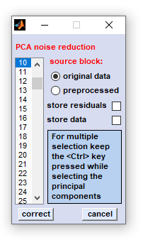
|
source block: select the source data block for noise correction store residuals: allows visualization of the residuals E which are separated from the noise corrected data when doing noise correction. The matrix of residuals E is copied into data block #4, the data block of deconvolution data. Note that this procedure may overwrite existing data of this type. store data: allows storing principal components and scores to a single file for later analysis (Matlab formatted) correct: starts the routine of PCA-based noise reduction cancel: the routine is aborted. Selections made are lost Important: Please carefully use this preprocessing routine! The decision which of the PCs can be omitted is highly subjective and may cause spectral artifacts. |
Parameters used for PCA-based noise correction are stored and are accessible through the
The algorithm has been inspired by a presentation given by Dr. Spragg R. (PerkinElmer) "Addressing Problems in Data Reduction for FT-IR Images of Biological Samples" at the meeting RISBM - Raman and IR spectroscopy in Biological Medicine, Feb 29 - Mar 02, 2004, Friedrich-Schiller-University, Jena, Germany.
Reference to the literature:
Cosmic Spike Correction
Raw data recorded by means of sensitive integrating detectors such as charged-coupled devices (CCD) commonly used in dispersive Raman
spectrometers may contain artifacts caused by high-energy cosmic particles hitting CCD detector elements. Such cosmic ray artifacts
manifest themselves as non-reproducible (random), sharp and intense features superimposed on the Raman signals. As these features can
corrupt important parts of the Raman spectra and mislead interpretation and / or subsequent multivariate analyses they are required to be
identified and replaced by a local estimate.
Cosmic spike removal: The cosmic spike correction function allows the user to remove cosmic ray features from experimental
hyperspectral Raman imaging data. CytoSpec's spike removal function is available from the 'Spectral preprocessing' menu bar.
When this function is chosen, a dialog box shows up which allows the user to change parameters of the cosmic spike correction function.
Algorithm of cosmic spike removal:
- Baseline correction: This optional feature allows baseline correction of the Raman spectra as a initial step of cosmic ray correction.
For this, the method baseline correction from minima is used
(Parameters: number of intervals: 13, unselected option 'interpolate spectral region').
- Smoothing of the hyperspectral data. Depending on the selection of source data (original, or preprocessed) and the status of
the checkbox 'smooth spectra', HSI data are smoothed either in the spectral, or the spatial dimension. Spectra are smoothed
by the Savitzky-Golay (SavGol) smoothing filter using n smoothing points in case of a activated checkbox 'smooth spectra'.
The number of smoothing points n can be chosen from the popupmenu '# smooth pts'. Alternatively, if the checkbox
'smooth spectra' is unchecked, HSI data are smoothed in the spatial domain, whereas a
n × n
SavGol smoothing kernel is employed with n denoting the pixel size of the kernel in x- and y-direction (popupmenu '# smooth
pts').
- The difference between the un-smoothed and smoothed HSI data is obtained.
- The resulting [x,y, λ] array of Raman difference intensity values is normalized by dividing its spectra by the noise level
derived for each individual pixel spectrum. Noise is obtained from signal-free spectral regions of the original data as the standard
deviation of Raman intensity values. Note that this procedure deviates from earlier CytoSpec implementations (before version 2.00.07)
where the noise level was determined from the complete HSI.
- Wavelength positions of 'cosmic spike candidates', i.e. of potential cosmic spike features, are now obtained for each individual
pixel spectrum by by a systematic analysis in the spectral domain. For this purpose, the resulting noise-normalized difference spectra
are analyzed: Raman shift positions with intensity values larger than the threshold value '10/sensitivity' are determined and added
to a list of cosmic spike candidates. The value of the parameter 'sensitivity' can be selected from the popupmenu 'sensitivity';
the higher the sensitivity the lower the intensity threshold and the larger the number of spike candidates.
- In the next step, spike candidates are systematically scanned on the basis of two criteria. The most relevant criterion is the
typical shape of cosmic spikes (sharpness). However, the frequency of spike candidates at certain Raman shift positions serves also as a
criterion: The more spike candidates are found at a given Raman shift position the lower is the probability that these features
are caused by cosmic rays, i.e. represent true spectral features).
- Raman pixel spectra which have passed checks for both criteria are finally corrected. Note that spike correction is applied to input data
of the correction function (steps 1-7 describe the methodology to identify and validate cosmic spike feature candidates!). Spike features
are removed by replacing Raman intensity values by average Raman intensity data obtained from from neighboring pixel spectra. The parameter
'spikes width' defines the width of spike features to be corrected in data point units.
- Cosmic spikes can be removed from original or preprocessed HSI data. In both cases spike-corrected Raman data are written into
the data block of preprocessed spectra. Note that existing preprocessed data are overwritten without warning.
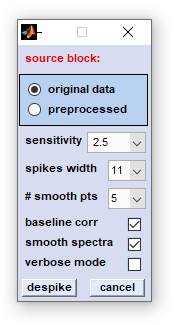
|
source block: allows selecting the type of source data
sensitivity: defines a threshold value for normalized difference Raman intensity values. Spectra [x,y] pixel coordinates and the Raman shift positions of features with a intensity larger than the threshold of '10/sensitivity' are added to a list of cosmic spike candidates. The higher the sensitivity the lower this threshold and the larger the number of spike candidates (see section algorithm for more details) spikes width: defines the width of the Raman shift region in which spike intensity values are replaced by mean intensity values from neighboring pixel spectra. # smooth pts (number of smoothing points): the number of smoothing points for SavGol smoothing in the spectral domain, or of the SavGol smoothing kernel, when data are smoothed in the image domain. baseline corr (baseline correction): optional baseline correction by the method of smooth spectra: determines the algorithm of how HSI data are smoothed (spectra, or image domain smoothing, see section algorithm for details) verbose mode: displays more details of cosmic spike correction function. despike: starts the procedure of cosmic spike correction. cancel: closes this dialog box. |
Cosmic ray correction parameters are stored and are accessible through the
Fourier Self-Deconvolution
Fourier self-deconvolution (FSD): The main purpose of Fourier self-deconvolution is to increase the apparent spectral resolution. The
procedure has been suggested in a series of publications by Kauppinen and coworkers (see below) as a band-narrowing, or resolution enhancement
technique. The FSD method decreases the effective line width, so that broad and overlapping band contours are separable. Mathematically,
FSD can be regarded a specific band pass filter consisting of a deconvolution function as the high pass filter and a smoothing or damping function
as the low pass filter. When applying FSD to real data one should be aware that the actual shape of the FSD filter function defines the degree
of band narrowing. Furthermore, FSD filter functions determine the shape of deconvolved bands and the degradation of the signal-to-noise ratio.
Inadequate FSD filter parameters (deconvolution factor, DF and noise reduction factor, NRF) may result in under- or over-deconvolution,
with the latter one characterized by noise amplification and the appearance of large negative side-lobes.
Note that Fourier self-deconvolution is only useful in cases where the vibrational bands are broader than the spectral resolution.
The procedure of Fourier self-deconvolution consists of the following sequence of steps:
- Experimental spectra are first Fourier-transformed.
- In the second step a exponential deconvolution function is obtained. For this the equations
y = exp(2*π*DF*x)
(Lorentzian line shape) or y = exp(2*π*DF*x²) (Gaussian) is employed. DF represents the deconvolution factor
while x denotes a vector of length N ranging from 0 to 1. N is the number of data points in the experimental spectrum.
- A damping function is determined by using the formula y = [1-abs(x)/NRF]². NRF is the noise reduction factor (see below for
details).
- The experimental Fourier-transformed spectrum (step 1) is multiplied by the exponential deconvolution function (step 2) and the damping
function (step 3).
- The resulting interferogram is back-transferred by an inverse Fourier transformation.
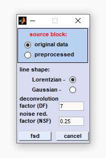
line shape: define the line shape by checking either the Lorentzian or Gaussian radio button. The line shape of bands in experimental spectra is determined by the type of line-broadening. In case of doubt start with the Lorentzian line shape (default setting). deconvolution factor (DF): The deconvolution factor represents a factor by which the vector of x-values is multiplied when obtaining the exponential deconvolution function. In case of Lorentzian line shapes the exponential function is obtained by the eqn. noise reduction factor (NRF): This factor should range from values > 0.0 to < 1.0. The NRF defines the fraction of the interferogram, at which the noise damping function reaches values of 0. A NRF value of 1 corresponds to the full interferogram length whereas a value of 0 means that the damping function equals zero at all interferogram points. Note that both values do not represent valid settings. Recommended values of NRF are 0.2 for Lorentz line shapes or 0.25 in case of a Gaussian shape. fsd: starts Fourier self-deconvolution of the data block selected. cancel: closes the dialog box. |
|
Reference to the literature:
Kramers-Kronig Transformation
Kramers-Kronig Transformation: to be continued
Batch Preprocessing
Batch preprocessing: This function permits automated preprocessing of hyperspectral image data. When this option is chosen one will
be asked to indicate a predefined macro file (*.cbt -CytoSpec batch) which should be generated (and tested!) beforehand.
CytoSpec batch files can be prepared by simple text editors like Wordpad, Notepad, or Notepad++. After compilation of *.cbt files it is
important to store them in a simple text format. Please do not use special characters or format tags.
CytoSpec batch preprocessing files are composed of individual text sections, or blocks, which sequence defines the sequence of preprocessing
steps carried out when using CytoSpec's automated preprocessing function ('batch preprocessing'). A text block always starts with one of
the following (capitalized) three-letter codes:
DER - Derivative
NOD - Node attenuation
NRM - Normalize
CUT - Cut / Crop
INT - Interpolate
SMO - Smoothing
TRA - TR → ABS conversion
ATR - ABS → TR conversion
SUB - Subtraction
QAL - Quality tests
LBS - Baseline correction (linear)
BAS - Baseline correction (SavGol)
BMI - Baseline correction from minima
ALS - Baseline correction by asymmetric least squares (AsLS)
WVC - Water vapor correction
PNR - PCA-based noise reduction
CSR - Cosmic spike correction
FFT - Fourier self-deconvolution (1-D case)
REP - Replace NaNs
BIN - Interpolate / binning (spatial)
FLT - Filter images
EPD - Edge-preserving denoising
FSD - 3D Fourier self-deconvolution
SWA - Swap data blocks
Video tutorial spectral and spatial preprocessing with CytoSpec (Youtube):
(in this video, utilization of the function 'batch preprocessing' is exemplified after position 5:50 min)
If a preprocessing function is not to be executed, the corresponding data block does not have to be deleted from the *.cbt macro file. In
these cases it is sufficient to comment out the first text line of the respective block, i.e. the line containing the three-letter code.
Outcommenting can be done by prepending the '#' (hash) character to this line. Furthermore, it is permissible to execute preprocessing
functions several times in succession, for example to normalize original and derivative data. The first line of a preprocessing text
block is followed by lines containing the complete set of parameters required for proper execution of the individual spectral or
spatial preprocessing function. These parameters are mandatory and must be provided by specially formatted text lines that start with
a three-letter code followed by either numeric values, or strings and a space character for separation. In these lines, comments can
be added afterwards but must be separated by at least one space character followed by the hash sign, please see examples below.
Comments are useful to specify individual preprocessing parameters and often provide allowed selection values of them, sometimes in
the following format: (5-7-9-11-13-15-17-19-21-23-25).
Note that each block has to be terminated by a line containing the code 'END'. Text lines that contain only hash signs, or with comments
after a hash sign can increase the readability of the batch code and can be inserted in any amount. Please refer also to the online
help or to the example file that comes with CytoSpec's installation CD / USB drive.
Example #1 of a block 'CUT' of a CytoSpec batch (*.cbt) file:
# --------------- CUT --------------------------------------------------
CUT
TYP 1 # type of cutting (1-spectral, 2 spatial dimension)
WV1 1000 # first frequency / wavenumber for cut in spectral dimension
WV2 1800 # last frequency / wavenumber (WV1 < WV2!)
XD1 1 # cut, spatial dimension x : first pixel to keep
XD2 10 # cut, spatial dimension x : last pixel to keep
YD1 1 # cut, spatial dimension y : first pixel to keep
YD2 10 # cut, spatial dimension y : last pixel to keep
END
# some lines with comments may follow
next block ...
Example #2 of a block 'CSR', Cosmic spike correction:
# --------------- COSMIC SPIKE CORRECTION -------------------------------
CSR
BLK 2 # type of source data block (1-original, 2-processed)
SNS 4 # sensitivity factor (0.5-0.8-1.0-2.0-2.5-3.0-4.0-5.0-6.0-8.0-10.0-12.0-15.0-20.0)
SKW 11 # spike width (5-7-9-11-13-15-17-21)
NSP 11 # number of smoothing points (5-7-9-11-13-15-17-19-21-23-25)
BSL 1 # perform baseline correction: 1-YES/0-NO
SMS 0 # smooth spectra (instead of images) 1-YES/0-NO
END
# some lines with comments may follow
next block ...
An example of a CytoSpec batch (macro) file with a description of all possible block types can be downloaded here:
preproc.cbt
NOD - Node attenuation
NRM - Normalize
CUT - Cut / Crop
INT - Interpolate
SMO - Smoothing
TRA - TR → ABS conversion
ATR - ABS → TR conversion
SUB - Subtraction
QAL - Quality tests
LBS - Baseline correction (linear)
BAS - Baseline correction (SavGol)
BMI - Baseline correction from minima
ALS - Baseline correction by asymmetric least squares (AsLS)
WVC - Water vapor correction
PNR - PCA-based noise reduction
CSR - Cosmic spike correction
FFT - Fourier self-deconvolution (1-D case)
REP - Replace NaNs
BIN - Interpolate / binning (spatial)
FLT - Filter images
EPD - Edge-preserving denoising
FSD - 3D Fourier self-deconvolution
SWA - Swap data blocks
# --------------- CUT --------------------------------------------------
CUT
TYP 1 # type of cutting (1-spectral, 2 spatial dimension)
WV1 1000 # first frequency / wavenumber for cut in spectral dimension
WV2 1800 # last frequency / wavenumber (WV1 < WV2!)
XD1 1 # cut, spatial dimension x : first pixel to keep
XD2 10 # cut, spatial dimension x : last pixel to keep
YD1 1 # cut, spatial dimension y : first pixel to keep
YD2 10 # cut, spatial dimension y : last pixel to keep
END
# some lines with comments may follow
next block ...
# --------------- COSMIC SPIKE CORRECTION -------------------------------
CSR
BLK 2 # type of source data block (1-original, 2-processed)
SNS 4 # sensitivity factor (0.5-0.8-1.0-2.0-2.5-3.0-4.0-5.0-6.0-8.0-10.0-12.0-15.0-20.0)
SKW 11 # spike width (5-7-9-11-13-15-17-21)
NSP 11 # number of smoothing points (5-7-9-11-13-15-17-19-21-23-25)
BSL 1 # perform baseline correction: 1-YES/0-NO
SMS 0 # smooth spectra (instead of images) 1-YES/0-NO
END
# some lines with comments may follow
next block ...
[
GENERAL |
FILE |
SPECTRAL PREPROCESSING |
SPATIAL PREPROCESSING |
UNIVARIATE IMAGING |
MULTIVARIATE IMAGING |
TOOLS |
FILE INFO |
GLOSSARY |
CONTACT: info@cytospec.com |
PUBLISHER DETAILS |
PRIVACY POLICY ]
Copyright (c) 2000-2026 CytoSpec. All rights reserved.
FILE INFO |
Copyright (c) 2000-2026 CytoSpec. All rights reserved.