CytoSpec - an APPLICATION FOR HYPERSPECTRAL IMAGING |
||||||||||||||||||||||||||||||


|
||||||||||||||||||||||||||||||
|
|
|
|||||||||||||||||||||||||||||
|
|
||||||||||||||||||||||||||||||
Menu Bar 'Multivariate Imaging' |
||||||||||||||||||||||||||||||
Create PCA maps from spectra |
||||||||||||||||||||||||||||||
HCA Image Segmentation |
||||||||||||||||||||||||||||||
Part II - Part III - HCA imaging: Part IV - |
||||||||||||||||||||||||||||||

 Load
Load 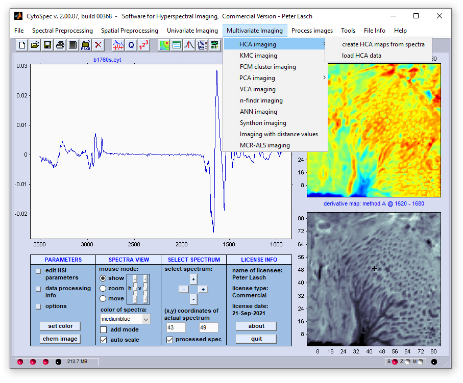
| Part I - Distance Matrix | 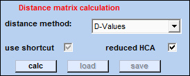 |
Given n objects, a distance or dissimilarity matrix, is a symmetric matrix with zero diagonal elements such that the ij-th element represents how far apart or how dissimilar the i-th and j-th objects are.
calc: starts the calculation of the distance matrix.
load: load distance matrix files (file extensions is '*.dis').
save: save the distance matrix.
use shortcut: if this option is chosen, the calculation of the distance matrix AND hierarchical clustering are queued that is no further user input will be required. Please select a distance AND a cluster method, even if the distance matrix has not been obtained, before pressing the 'calc' button. Note also that the distance matrix cannot be stored when this option was selected.
reduced HCA: This HCA imaging option is particularly useful when large data sets are analyzed. It is recommended to choose this option for data files containing more than 128 × 128 spectra. In reduced HCA, the calculation of the distance matrix and hierarchical clustering are carried out on the basis of randomly selected spectra. When finished, mean cluster spectra of the last 50 clusters are obtained. Then,n × 50 distance values between all spectra and mean cluster spectra are obtained (n is the number of pixel spectra in the data set). Cluster memberships are then assigned on the basis of these distance values. Please note, that 'reduced HCA' is available only for the distance option 'D-values'.
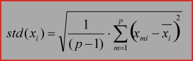
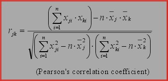
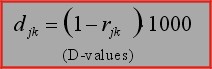
distance method: pop up menu which allows to select one of the following methods for distance matrix calculation.
1. D-Values
2. Euclidean distances 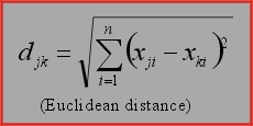
3. Normalized Euclidean distances 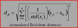
4. Euclidean squared distances 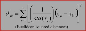
5. City block. 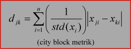
| Part II - Hierarchical clustering | 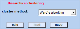 |
calc: starts hierarchical clustering.
load: load cluster analysis files. The file extension is '*.cls'.
save: save cluster analysis results.
cluster method: here you can select a method for clustering:
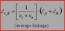
1. Average linkage
2. Single linkage 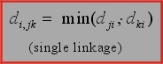
3. Complete linkage 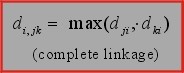
4. Group average 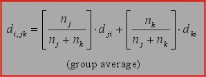
5. Centroid method. 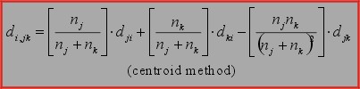
6. Median algorithm 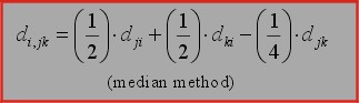
7. Ward's algorithm 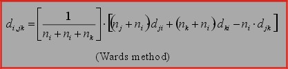
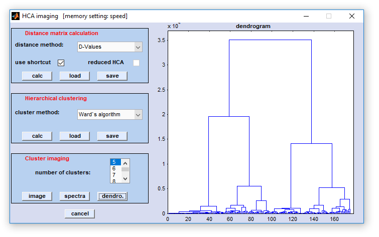
| Part III - HCA imaging | 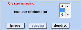 |
number of clusters: allows selection of the number of clusters used for HCA imaging. Minimum is 2, maximum: 50.
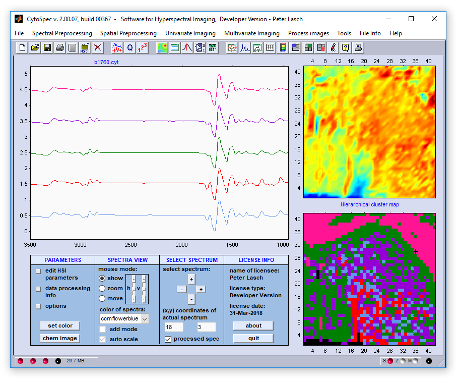
image: displays the HCA segmentation map. The number of classes (clusters) are color encoded. The color sequence is determined by the active color map, usually the color map 'ann' (see functionDisplay Spectra).
dendro: A dendrogram is shown on the display. The dendrogram can be stored as bitmap ('*.bmp') or as an encapsulated postscript ('*.eps') data file. Both functions are available by a activating the context menu of the dendrogram axis. Note that dendrograms will display only the last 500 fusion steps.
spectra: this function produces and displays cluster mean spectra. After clicking on the 'spectra' button, a dialog box for choosing the source data block comes up. The selected data block is used to obtain and display cluster mean spectra. Details of the function can be found in the section
Part IV - An example of HCA image segmentation:
Reference to the literature:

KMC Image Segmentation - k-Means Cluster Imaging
Principles of k-means clustering: The algorithm of k-means clustering has been suggested by J.B. MacQueen in 1967:
J.B. MacQueen. In L.M. LeCam and J. Neymann (eds) Proceedings of Fifth Berkeley Symposium on Mathematical
Statistics and Probability. 1967 281-297.
Related web links (Wikipedia):
k-means clustering
k-means algorithm
In the CytoSpec implementation, MacQueens k-means cluster algorithm is used. k-means clustering is a non hierarchical clustering
method, which obtains a "hard" (crisp) class membership for each spectrum, that is the class membership of an individual spectrum
can be taken only the values of zero or one. It uses an iterative algorithm to update randomly selected initial cluster centers, and
to obtain the class membership for each spectrum, assuming well-defined boundaries between the clusters. MacQueens iterative algorithm
of KMC can be described as follows: Spectra are illustrated as points in a p-dimensional space (p is the number of features of the
spectra. In this space a number of k points is initially chosen, where each point represents a cluster to be made. Then, distance
values between the points and all objects (spectra) are calculated. Objects are assigned to a cluster on the basis of a minimal distance
value. Next, centroids of the clusters are calculated and distance values between the centroids and each of the objects are re-calculated.
Then, if the closest centroid is not associated with the cluster to which the object currently belongs, the object will switch its cluster
membership to the cluster with the closest centroid. The centroid's positions are re-calculated every time a component has changed the
cluster membership. This continues until none of the objects has been re-assigned.
Data selection: After selection of the function 'KMC imaging' a standard dialog box entitled 'k-means clustering'
comes up. This dialog box allows selecting up to four non-overlapping spectral regions from the data block of
choice, see help chapter data selection for multivariate imaging for further
details.
Once data selection has been completed, the following dialog box will appear:
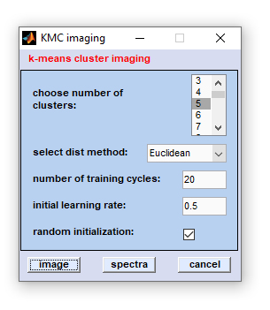
How to start KMC imaging? Once data preparation has been finished, the KMC imaging dialog box appears. Indicate how many
classes are assumed to be present in the data set ('choose number of cluster') and the enter the 'number of training cycles'
(default: 20). Furthermore it is required to select an 'initial learning rate' (default 0.5) and a method to obtain interspectral
distances. KMC imaging can be carried out using the following distance methods: Euclidean, standardized Euclidean, D-values (normalized
Pearsons's correlation coefficients), and PCA. PCA means Euclidean distances in PCA space (first 12 principal components). KMC is usually
done by a random initialization of the centroids. Please uncheck the checkbox 'random initialization' if you don't want this.
To start the KMC imaging function hit the 'image' button, to exit press 'cancel'. When the calculation is finished the
cluster map will be immediately plotted in the axis of the preprocessed maps using the colormap 'ann'.
spectra: this function produces and displays k-means cluster mean spectra. After clicking on the 'spectra' button,
a dialog box for choosing the source data block comes up. The selected data block is used to obtain and display cluster mean
spectra. Details of the function can be found in the section
multivariate imaging - dialog box 'spectra' of the CytoSpec help pages.
Reference to the literature:
Lasch P, Hänsch W, Naumann D, Diem M.
Imaging of colorectal adenocarcinoma using FT-IR microspectroscopy and cluster analysis. Biochim Biophys Acta. 2004
1688(2):176-86.
FCM Cluster Image Segmentation - Fuzzy C-Means Cluster Imaging
Related web links:
fuzzy C-means clustering
(Wikipedia)
The principles of fuzzy C-means clustering are given in the following publication:
J.C. Bezdek. Pattern Recognition with Fuzzy Objective Function Algorithms, 1981 New York. Plenum Press.
FCM clustering is a non hierarchical clustering method. This clustering technique partitions objects into groups (cluster) whose members show
a certain degree of similarity. Unlike k-means clustering, the output of FCM clustering is a membership function, which defines the degree of
membership of a given spectrum to the clusters. The values of the membership function can vary between one (highest degree of cluster
membership) and zero (no class membership), where the sum of the C
cluster membership values for one object equals one.
Thus, this method departs from the classical two-valued (0 or 1) logic, and uses "soft" linguistic system variables and a continuous range
of true values in the interval [0,1]. FCM imaging uses a fuzzy iterative algorithm to calculate the class membership grade for each spectrum.
The iterations in FCM clustering are based on minimizing an objective function, which represents the distance from any given data point
(spectrum) to the actual cluster center weighted by that data points membership grade.
The advantage of the fuzzy C-means clustering over k-means clustering is that both outliers and data, which display properties of more than
one class can be characterized by assigning nonzero class membership values to several clusters. In the similarity maps assembled by FCM
clustering the membership values are encoded by the colormap, that is by the color intensities in the case of single color colormaps.
Data selection: After selection of the function 'FCM cluster imaging' a standard dialog box entitled 'fuzzy C-means
clustering' comes up. This dialog box allows selecting up to four non-overlapping spectral regions from the data block of
choice, see help chapter data selection for multivariate imaging for further
details.
Once data selection has been completed, the following dialog box will appear:
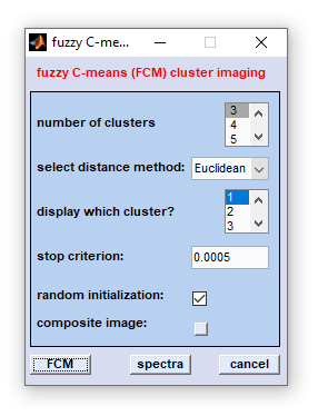
How to start FCM imaging? Once data preparation has been finished, the FCM imaging dialog box appears. Indicate how many classes
are assumed to be present in the data set ('number of clusters') and give an exit criterion ('stop criterion', default:
0.0005). Furthermore it is required to select a method to obtain interspectral distances. FCM imaging can be carried out using the
following distance methods: Euclidean, standardized Euclidean, D-values (normalized Pearsons's correlation coefficients), and PCA.
PCA means Euclidean distances in PCA space (first 12 principal components). FCM is usually done by a random initialization of the cluster
centers. Please uncheck the checkbox 'random initialization' if you don't want this.
To start the FCM imaging function hit the 'FCM' button, to exit press 'cancel'. When the calculation is finished select a
cluster that should be used to reassemble the image ('display which cluster'). The single cluster image is plotted in the axis of
the preprocessed maps using the colormap 'black'. A composite image can be created in a separate window by pressing the button 'composite
image'.
spectra: this function produces and displays fuzzy C-means cluster mean spectra. After clicking on the 'spectra' button,
a dialog box for choosing the source data block comes up. The selected data block is used to obtain and display cluster mean
spectra. Details of the function can be found in the section
multivariate imaging - dialog box 'spectra' of the CytoSpec help pages.
composite image: Creates a composite image from the cluster membership functions. A detailed description of the functionality is provided in
section composite images of CytoSpec's online documentation.
Reference to the literature:
Lasch P, Hänsch W, Naumann D, Diem M. Imaging of
colorectal adenocarcinoma using FT-IR microspectroscopy and cluster analysis. Biochim Biophys Acta. 2004 1688(2):176-86.
PCA Imaging - Imaging Using Principal Component Analysis
Principles of PCA: PCA is a linear transformation in which the (spectral) data are transferred into a new coordinate system. In
this new coordinate system, the largest data variance points to the direction of the first coordinate, which is also called the first
principal component (pc), the second largest variance on the second pc, and so forth. PCA can be thus considered a transformation that
re-arranges the data according to the data's intrinsic variance: most of the variance is contained in the lower-order principal components
while higher-order pc's are supposed to contain mainly noise. Reduction of dimensionality by PCA can be effectively achieved by omitting
higher-order principal components.
Related web links (Wikipedia):
Principal Component Analysis
Data selection: After selection of the function 'PCA imaging' a standard dialog box entitled 'principal component
analysis' comes up. This dialog box allows selecting up to four non-overlapping spectral regions from the data block of
choice, see help chapter data selection for multivariate imaging for further
details.
Once data selection has been completed, the following dialog box will appear:
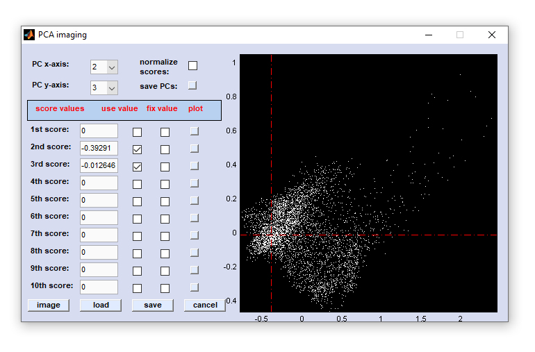
How to start PCA imaging: One can start the PCA imaging function either from the 'Multivariate Imaging → PCA imaging →
create PCA maps from spectra' menu or from the menu bar 'Multivariate Statistics → PCA imaging → load PCA data'. In
the latter case one have to load a PCA file (*.pca) obtained in earlier program sessions. Please refer to the chapter
Multivariate Statistics → PCA imaging → create PCA maps from spectra
if you want to produce PCA images directly from a hyperspectral data set.
Define the number of dimensions: to specify which PCs should be used for imaging, check the appropriate checkboxes of the column
'use value'. In the example above the principal components one and two are activated. The CytoSpec program permits the use of the
first 10 principal components.
Definition of individual score coefficients: first, select the principal components to be displayed from the popup menus in the upper
part of the PCA imaging window (PC x- or y-axis). Then, click into the score plot window to the right. The respective coordinates of this
action are transferred to the edit fields indicated as 1st to 10th score. Alternatively, it is possible to manually type the respective
coordinates into these boxes.
Normalization of the score coefficients: checking the checkbox 'normalize scores' causes normalization of distances between score
coefficients and 'mass centers' such that the maximum distance for all principal components equals one.
save PCs: if this option is chosen, the first 10 principal components are stored (see description of the button 'save' below
for details).
What does 'fix value' mean? This option permits to fix the coordinates of a given mass center in the n-th dimension, irrespective
of mouse manipulations in the plot to the right. This option may be useful when searching for an optimal contrast of a PCA image.
What happens if one of the buttons 'plot' is pressed? In this case all scores coordinate centers are set to zero and a PCA
image using the i-th score coefficients is produced (i.e. the i-th score coefficients are linearly converted into color scales).
imaging: using the actual coordinates of the mass centers, PCA images are plotted into the lower right panel of the main window.
load: opens a standard window for opening files of the format *.pca.
save: allows to save score coefficients and principal components. File extension will be *.pca. If the checkbox 'save PC's'
was checked, the first 10 principal components are stored as separate double column ASCII files. These files are stored in the same
directory as the *.pca-file.
cancel: closes the PCA imaging window. Data not stored are lost.
Note that spectra with negative Quality Test results, or
unselected Regions of Interest are excluded from the analysis and appear
in PCA images as black pixels.
Reference to the literature:
Lasch, P. & Naumann, D. FT-IR Microspectroscopic Imaging of
Human Carcinoma Thin Sections Based on Pattern Recognition Techniques. Cellular and Molecular Biology 1998 44(1). pp.
189-202
VCA Imaging - Imaging Using Vertex Component Analysis
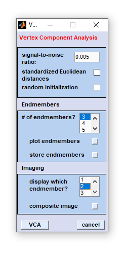
Principles of VCA: VCA (vertex component analysis) is an unsupervised method to rapidly unmix hyperspectral data. The algorithm
was initially developed by J. Nascimento and J. Dias. The idea of VCA can be summarized as follows: Given a set of mixed spectral
(multispectral or hyperspectral) vectors, linear spectral mixture analysis, or linear unmixing, aims at estimating the number of reference
substances, also called endmembers, their spectral signatures, and their abundance fractions. Unsupervised endmember extraction by VCA
exploits the following facts: the endmembers are the vertices of a simplex and the affine transformation of a simplex is also a simplex.
Furthermore, VCA assumes the presence of pure pixels in the data. The algorithm iteratively projects data onto a direction orthogonal to
the subspace spanned by the endmembers already determined. The new endmember signature corresponds to the extreme of the projection. The
algorithm iterates until all endmembers are found.
Related publications:
J. Nascimento and J. Dias, "Vertex Component
Analysis: A fast algorithm to unmix hyperspectral data", IEEE Transactions on Geoscience and Remote Sensing 2005 vol. 43,
no. 4, pp. 898-910
Unsupervised unmixing of hyperspectral imagery using the constrained positive matrix factorization by Yahya M.
Masalmah. July 2007. Dissertation, University of Puerto Rico. Chair: Miguel Velez-Reyes, Major Department: Computing and Information
Science and Engineering
Data selection: After selection of the function 'VCA imaging' a standard dialog box entitled 'vertex component
analysis' comes up. This dialog box allows selecting up to four non-overlapping spectral regions from the data block of
choice, see help chapter data selection for multivariate imaging for further
details.
Once data selection has been completed, the following dialog box will appear:
|
|
Application example of imaging by VCA in vibrational hyperspectral imaging:
n-findr Imaging - Imaging Using the n-findr Endmember Extraction Technique
Theory - related links
M. E. Winter. N-FINDR: an algorithm for fast autonomous
spectral end-member determination in hyperspectral data. volume 3753, pages 266-275, Denver, CO, USA, October 1999. SPIE.
Winter, Michael E., "Fast Autonomous Spectral End-member Determination In Hyperspectral Data", Proceedings of the Thirteenth International
Conference on Applied Geologic Remote Sensing, Vol. II, pp 337-344, Vancouver, B.C., Canada, 1999.
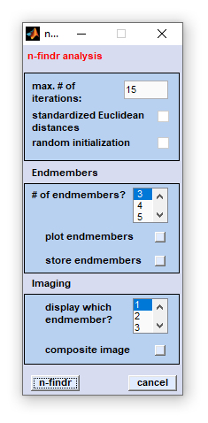
Data selection: After selection of the function 'n-findr imaging' a standard dialog box entitled 'n-findr
analysis' comes up. This dialog box allows selecting up to four non-overlapping spectral regions from the data block of
choice, see help chapter data selection for multivariate imaging for further
details.
Once data selection has been completed, the following dialog box will appear:
Winter, Michael E., "Fast Autonomous Spectral End-member Determination In Hyperspectral Data", Proceedings of the Thirteenth International Conference on Applied Geologic Remote Sensing, Vol. II, pp 337-344, Vancouver, B.C., Canada, 1999.
|
|
Application of n-findr imaging in vibrational hyperspectral imaging:
ANN Image Segmentation - Imaging Using Artificial Neural Networks
This function of the CytoSpec program has been originally designed to re-assemble hyperspectral images on the basis of classification results
of artificial neural networks (ANN) classifiers. In this function, result files (*.res) of the Stuttgart Neural Network Simulator (SNNS)
are analyzed and directly converted into false-colored ANN segmentation images. Furthermore, checks for activation thresholds and multiple
activations can be carried out.
Note that the SNNS and its successor JavaNNS are now outdated and are no longer maintained. Therefore, utilization
of more advanced network simulators is highly recommended. However, to ensure compatibility of CytoSpec with older SNNS network models also for the
future, the CytoSpec-SNNS interface function will remain a part of future program versions. Nevertheless, it is recommended not to start new projects
that make use of this interface.
The SNNS was developed at the "Institut für Parallele und Verteilte Höchstleistungsrechner" (IPRV) of the Universität Stuttgart
(Germany). The SNNS is still available and can downloaded for free at
ftp://ftp.informatik.uni-stuttgart.de.
A tutorial of how to use the CytoSpec-SNNS interface is given here
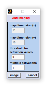
|
map dimensions (x): the number of measurement positions in x-direction.
|
Please check also the format of the SNNS result files. The *.res file should have the following format: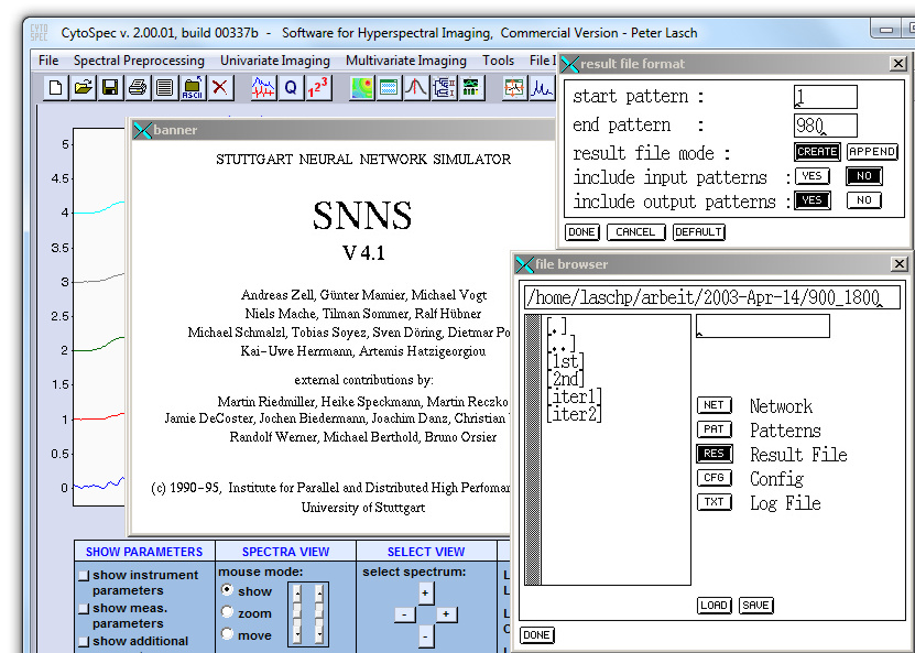
In the example given above, 980 spectra obtained from a rectangular area (20 × 19 spectra) were analyzed. The number of pre-defined classes in the teaching phase of ANN model development equals 4.SNNS result file V1.4-3D
generated at Tue Mar 25 11:24:47 1997
No. of patterns : 980
No. of input units : 76
No. of output units: 4
startpattern : 1
endpattern : 980
teaching output included
#1.1
1 0 0 0
0.06227 0.82028 0.01888 0.00005
#2.1
1 0 0 0
0.97587 0.35621 0.00001 0.00089
#3.1
1 0 0 0
0.99435 0.28643 0.00001 0.00046
.....
#979.1
1 0 0 0
0 0.05502 0.98514 0.21558
#980.1
1 0 0 0
0 0.14128 0.81746 0.61632
The first line of the first pattern (#1.1) shows the a priori class assignment (target pattern), while the second line displays the ANN test results for this particular spectrum. The maximum activation was found for the second output neuron (0.82028), indicating a posteriori class assignment of this individual spectrum to class # two. CytoSpec automatically analyzes the posteriori assignments for all spectral sub-pattern contained in the *.res file and assigns specific colors to each class. Images are produced by combining colors with spatial (pixel) positions of the spectra assuming rectangular regions and equal distances between pixels in x- and y-direction, respectively.
The following types of ANNs were tested to be compatible:
- multilayer perceptron (MLP) networks consisting of three layers of neurons (input layer, hidden layer, output layer)
- ANNs with feed-forward propagation of activations, shortcut connections are allowed
- teaching functions: backpropagation, resilient backpropagation (rprop), quickpropagation (quickprop)
Reference to the literature:
Image Segmentation with Synthon's NeuroDeveloper™ Neural Network Simulator
The function 'Synthon imaging' represents basically an interface between CytoSpec and Synthon's
NeuroDeveloper™, a simulator for teaching and validating artificial neural network models by spectra of various origins (e.g. IR, Raman,
MS spectra). Based on neural network models, the interface can be used to re-assemble ANN images from CytoSpec's original data sets. Spectral
preprocessing, features extraction and ANN classification of a priori unassigned HSI data sets can be conveniently performed This is achieved by
utilizing the runtime environment of the NeuroDeveloper™ software which does not require a software license from Synthon. Spectral data can be
therefore classified without the NeuroDeveloper™ software on the basis of predefined network models. The NeuroDeveloper™ software is only
required in cases where new neural network models are needed.
Synthon GmbH, contact address:
Analytics and Pattern Recognition
Im Neuenheimer Feld
69120 Heidelberg
GERMANY
phone: +49 6221 50 257 900
fax: +49 6221 50 257 909
email: info@synthon-analytics.de
internet: http://www.synthon-analytics.de

To start the function select 'Synthon maps' from the 'Image manipulation' menu bar:
Synthon GmbH, contact address:
Analytics and Pattern Recognition
Im Neuenheimer Feld
69120 Heidelberg
GERMANY
phone: +49 6221 50 257 900
fax: +49 6221 50 257 909
email: info@synthon-analytics.de
internet: http://www.synthon-analytics.de
|
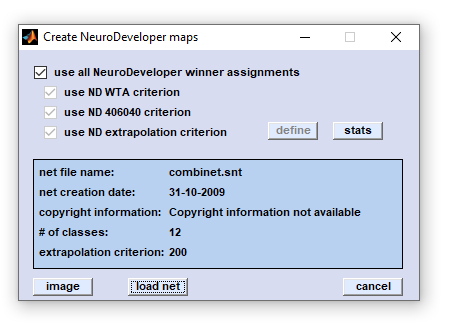
load allows to browse the directory structure and load the NeuroDeveloper™ network library (*.snt) file. After loading the
'image' and 'stats' buttons become activated.
|
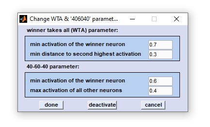
Evaluation of the activations calculated by the network model is performed by means of analysis functions like WTA and 40-20-40. In these evaluations the scores and the distribution of activation values of output neurons are taken into account.
'WTA' criteria:
WTA stands for winner takes all, which means classification depends on the highest output activation. A spectrum will only be classified if one of its activation values is larger than the defined minimum activation of winner neuron (default 0.7) AND if the minimum distance to the second highest activation is larger than 0.3 (default). Otherwise the classification will not be considered correctly and the spectrum remains unclassified.
'406040' criteria
The 40-20-40 function works differently. The activation of one neuron has to exceed 0.6 (default, above 60 percent of the activation range). All other activations of further classes have to be below 0.4 (below 40 percent of the activation range). Otherwise, the spectral pattern remains unclassified.
'extrapolation'' criterion
A general problem with different classification methodologies is the potential misclassification due to undesired or unexpected extrapolation. This occurs, when the training and validation data sets do not comprise all classes or the entire range of a feature needed for a given classification problem. In this case, any classification method, including ANNs, would not be representative for the given problem. Data of this type should rather be termed 'not classified'. The NeuroDeveloper™ uses a distance value derived from the training and validation data sets to determine an extrapolation problem. The maximum distance of a pattern to its corresponding class is calculated and set to 100. During the classification of a new pattern by the ANN, the distance of the new pattern is calculated and set into relation. In case the calculated extrapolation value of the class, identified by the neural network, exceeds 100, an extrapolation occurs. The default value to determine patterns as unclassified is proposed to be set to 200. The value should be set greater than 100, the smaller the value, the stricter the threshold.
Please note: If the checkbox 'use NeuroDeveloper™ winner assignments' was checked, CytoSpec does not perform an analysis of the WTA, 406040 and extrapolation results. The NeuroDeveloper™ software excludes spectra from further analysis in the following way:
- either both, the WTA, AND the 406040 criteria,
- or classification based on the extrapolation criterion failed.
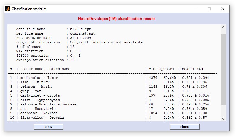
Screenshot of the NeuroDeveloper™ classification statistics window:
A. Compilation of data sets for teaching and internal validation
| 1. | Load an HSI set and produce any image (e.g. chemical image, UHCA segmentation image) |
| 2. | Obtain the context menu of image by clicking with the right mouse button over the false color image. |
| 3. | Choose 'class 1' → and 'start' if you intend assigning spectra to class 1. Now, you are in the 'select spectra' mode. In this mode, the mouse cursor changes its appearance (arrow plus cross). |
| 4. | You can select now an unlimited number of spectra by left mouse clicks (in this mode; spectra will be not displayed). The spatial coordinates will be given in the command line window. |
| 5. | To stop the selection mode, choose 'selection mode off' from the context menu. Alternatively, you can immediately start to assign spectra to class 2 by selecting 'class 2' → and 'start' from the context menu. In this way, spectra can be assigned to up to 8 distinct classes. |
| 6. | If all spectra are selected, stop the selection mode by 'selection mode off'. In the normal 'show spectra' mode the mouse pointer will regain its normal appearance (arrow). |
| 7. | In order to export spectra select the 'export' → 'x,y ASCII' from the 'File' menu bar. A window with the title 'convert into a (x,y) ASCII data format' appears. Check the checkbox 'export selection'. Please use the default settings for all other options. Make sure, that the data block of original absorbance spectra is exported. |
| 8. | Press button 'export' and store the spectra in a folder of your choice. Spectra of class 1 can be identified by the extension '*_1.dat', spectra by class 2 are named '*_2.dat' and so forth. |
| 9. | Steps 1-8 should be repeated for a number of maps. It is recommended to use consistent class assignments for identical (histological) structures. |
| 10. | Subdivide the spectral data into a subset for teaching (ca. 65 % of the spectra) and internal validation (35%) |
Now you can load the spectral data into the NeuroDeveloper™ software. Perform class assignment and preprocessing. Teach and validate the ANNs and store the network (see Synthon's NeuroDeveloper software manual for details).
The network file (*.snt) contains all relevant information for preprocessing and classification. This file, and Synthon's run-time environment (NOT the NeuroDeveloper™) are required for classification.
B. Produce NeuroDeveloper™ segmentation images (e.g. for external validation)
| 1. | Load a HSI. It is recommended to produce first a chemical image from the data block original spectra. |
| 2. | Select 'Synthon images' from the 'Multivariate imaging' menu bar. A window entitled ' create NeuroDeveloper™ images' will appear. Press the 'load' button and select one of NeuroDeveloper's™ network files (*.snt). |
| 3. | Spectra from the data block of original data are now written to a temporary file, please make sure there is sufficient free disk space. Data are then preprocessed and classified by Synthon's run-time library. After this, the classification results are automatically imported by CytoSpec. When finished the button 'image' becomes activated. Press this button to display the NeuroDeveloper™ segmentation map. If you wish to modify the NeuroDeveloper™ exclusion criteria such as WTA, 406040, or extrapolation, uncheck the respective checkboxes and press 'define'. Then change parameters and close the dialog box. Press 'image' to apply the new definitions. Classification statistics are available by pressing the 'stats' button of the 'create NeuroDeveloper™ image' figure (see screenshot above for an example). |
Selected references to the literature:
Imaging with Distance Values
Principles of the function: This multivariate imaging method uses multivariate distances obtained between predefined internal, or external
reference spectra and spectra of the the current hyperspectral image (HSI). Various types of distance values can be systematically calculated from
the chosen reference spectra and all spectra of the HSI. Resulting arrays of distance values (Euclidean, D-values, etc.) are of dimensions
[xdim, ydim] with xdim representing the number of spectra in x-direction and ydim being the number of spectra in y-dimension. Distances are
subsequently color scaled and individual 'distance images', or image layers are produced by plotting specifically colored pixels as
functions of their spatial coordinates. Up to six differently colored distance image layers can be generated, manipulated and finally overlaid to
produce a so called 'composite image'.
Mathematical distances - related web links
Distance (Wikipedia)
Data selection: After selection of the function 'Imaging with distance values' a standard dialog box entitled 'imaging with
interspectral distances' comes up. This dialog box allows defining the source data block. Unlike other multivariate imaging functions,
the standard dialog box does not offer selecting spectral regions as inputs, see help chapter
data selection for multivariate imaging for more details.
Once data selection has been completed, the following dialog box will appear:
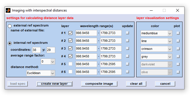
Dialog box 'Imaging with distance values'
external ref spectrum: activate first this radio button to load / import an external double column ASCII reference spectrum. For spectra
import press then the button 'load spec' and chose the external spectrum file. The directory and the file name will be displayed
afterwards. Press 'create new layer' to obtain distances between the external reference spectrum and spectra of the current HSI and
to produce a distance image (gray-scale image).
name of external file: indicates the name and path of the current external reference spectrum
internal ref spectrum (default): interspectral distances and distance image layers are produced using an internal reference spectrum
extracted from the current HSI. The spatial [x,y] coordinates of this internal spectrum are displayed by the following two edit fields:
x-coordinates: and y: coordinates of the internal reference spectrum can be modified, either manually, or by a left mouse click
into into a predefined chemical image.
average range factor: a value of 1 indicates that only the pixel spectrum at the [x,y] coordinates indicated is utilized as the internal
reference spectrum. If an average spectrum from the current [x,y] pixel spectrum and its immediate neighbors is to be used, then select a
value of 2. Select correspondingly larger values (2 or 3) if more distant neighbor spectra are to be considered. This option is useful for
distance imaging with noisy reference spectrum data.
When done press 'create new layer' to obtain distances between the internal reference spectrum and spectra of the current HSI and to
produce a distance image (gray-scale image).
distance method: defines the type of interspectral distances to be used for imaging: Euclidean (2-norm), standardized Euclidean, Manhattan
distance (1-norm) and and D-values (based on normalized Pearson's correlation coefficients).
further settings for calculating distance layers data. The function 'imaging with distance values' allows to produce up to six
individual distance images. Each of these images can be considered a layer of a so-called composite image that is produced by
superimposing individual distance images. The following gui elements are arranged in six lines whereas each line of elements can be used
to define settings for an individual distance image layer:
checkbox layer: allows to remove the current image layer data
edit field wavelength range(s): These fields allow to define the spectral ranges for calculating the distance values. Note that
different spectral windows can be used for the different layers. Furthermore, more than just one spectral window can be defined. For
example, to employ data from two spectral windows (950 - 1800 cm¹ and 2800 - 3000 cm¹) indicate '950; 2800' in edit
field 1 and '1800; 3100'' in field 2.
button update: by pressing this button all parameters are re-read and utilized to construct the current image layer. Please consider
that this always involves also the current settings for using an internal / external spectrum and includes also the indicated [x,y] pixel
spectrum coordinates. It is recommended to check all parameters of the active image layers by the tooltip content displayed over the respective
'#' character (hash sign)
popup menu color: allows definition of the color of the individual distance layer. Colors are pre-defined based on the settings
made in the file color.txt (see color.txt for details.
button plot: plots the current distance layer image in the true spatial aspect ratio using the predefined color.
load spec: becomes active only if the checkbox 'external ref spectrum' has been activated. Permits to load the external reference
spectrum (double column ASCII).
create new layer (button): interspectral distances between an internal/external reference spectrum and the HSI spectra are obtained.
Distances are employed to produce a single distance image which is plotted in the axis of preprocessed images (main window) whereas the
colormap 'black' is used.
composite image (button): a composite image is produced from all image layers defined so far. A detailed description of this
functionality is provided in section composite images of
CytoSpec's online documentation.
clear data (button): all layers are cleared from the CytoSpec workspace.
cancel (button): press this button to exit.
edit field wavelength range(s): These fields allow to define the spectral ranges for calculating the distance values. Note that different spectral windows can be used for the different layers. Furthermore, more than just one spectral window can be defined. For example, to employ data from two spectral windows (950 - 1800 cm¹ and 2800 - 3000 cm¹) indicate '950; 2800' in edit field 1 and '1800; 3100'' in field 2.
button update: by pressing this button all parameters are re-read and utilized to construct the current image layer. Please consider that this always involves also the current settings for using an internal / external spectrum and includes also the indicated [x,y] pixel spectrum coordinates. It is recommended to check all parameters of the active image layers by the tooltip content displayed over the respective '#' character (hash sign)
popup menu color: allows definition of the color of the individual distance layer. Colors are pre-defined based on the settings made in the file color.txt (see
button plot: plots the current distance layer image in the true spatial aspect ratio using the predefined color.
MCR-ALS Imaging - Imaging by Multivariate Curve Resolution - Alternating Least Squares
Principles of MCR-ALS: The term MCR-ALS (Multivariate Curve Resolution - Alternating Least Squares) is commonly used to denote a group
of techniques designed to recover pure response profiles (spectra, concentration, time, elution profiles, etc.) of chemical constituents of
an unresolved mixture. In hyperspectral imaging application MCR-ALS assumes that all pixel spectra constituting a HSI can be considered
linear combinations of pure component spectra. In this way each of the components is weighted by its concentration at any given [x,y]
position of the pixel spectrum. MCR-ALS imaging is an iterative procedure that aims at finding the pure component spectra as well as the
corresponding (spatial) concentration profiles of the components. This is achieved solely on the HSI data and one important input parameter,
the number of components.
Details of the MCR-ALS theory and applications can be found in the literature (see link below and at the end of this section)
Video tutorial MCR-ALS imaging with CytoSpec (Youtube):
Related web resources (Multivariate Curve Resolution Homepage):
Webpage of the MCR-ALS method with programs, tutorials
and data sets
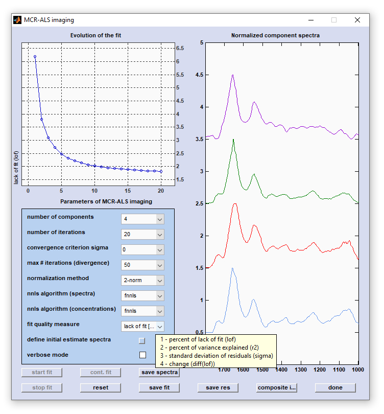
Screenshot of the figure 'MCR-ALS imaging' with the panel 'Evolution of the fit' (top right) and the panel to display
initial
estimate spectra, or optimized spectra components (left).
How to start MCR-ALS imaging? MCR-ALS imaging can be started from the menu bar 'Multivariate Statistics → MCR-ALS imaging'.
This will open CytoSpec's standard window for data preparation of multivariate imaging approaches, such as HCA, PCA, VCA, KMC imaging, etc.
In this window select the appropriate data source block - mostly original, or preprocessed data - and indicate the number of spectral
windows with the respective values of the wavelength, or frequency regions. Note that these spectral regions must not overlap.
To proceed press button labeled 'MCR-ALS'.
number of components: one of the most important setting of the MCR-ALS fit procedure. In case of doubts what what will be the optimal
number of components it is recommend to test different values. Alternatively, functions like
hierarchical clustering (analysis of the dendrogram!),
PCA imaging or
VCA imaging could be helpful to get an idea on suitable values for this parameter.
Note that changing the number of components will delete the results of the current fit session. Initial estimate spectra will be
initialized on a random basis (re-initialization).
number of iterations: MCR-ALS uses an iterative procedure to determine the component spectra and their concentration profiles. This
popup menu allows defining the maximum number of allowed iterations which might be useful to reduce computational efforts in case of
large HSI data sets. Note that changing this parameter will result in re-initialization.
convergence criterion sigma: the progress of the optimization procedure is monitored at each iteration cycle by a number of fit
quality measures parameters (lack of fit [%] - lof, and some others, see below for details). The change of the lof parameter between
two consecutive iterations is described by the parameter 'change'. This parameter is positive if the fit is improving and
negative in case of a not improving fit.
The convergence criterion 'sigma' is represents a threshold for the parameter
'change' and defines of whether to proceed or to leave the iterational procedure: Iteration will be stopped if the modulus of
'change (fit improvement) is equal or smaller than 'sigma'. Changing this parameter will re-initialize the fit session.
max # iterations (divergence): this divergence criterion is defined as the maximum number iteration cycles at which 'lof'
is allowed to grow. Optimization is aborted if 'lof'' has not decreased during the last n number of iterations.
Changing the divergence criterion parameter will re-initialize the fit session.
normalization method: select which type of normalization of the component spectra is used at each step of the MCR-ALS fit
procedure. Available options are 'no normalization' (not recommended, for testing only), '1-norm', '2-norm'
(default), 'maximum norm', 'offset correction', 'SNV' (standard normal variate, not recommended,
suitable only derivative spectra) and 'vector norm' (only for derivative spectra, not recommended for non-negative component
spectra). Changing the method of normalization will cause re-initialization of the fit session.
For details of the normalization algorithms please refer to
normalization.
nnls algorithm (spectra): defines the algorithm to solve the regression problem of the spectra components. Valid options are
'1 - not used', '2 - cut negative', '3 - lsqnonneg' and '4 - fnnls' as the default option. Option 1
('not used'') is only recommended for working with derivative spectra - it cancels the non-negative constraint of MCR-ALS
while option 2 ('cut negatives'') is applicable in some cases for reducing computational efforts - unconstrained estimation
is used and negative values are simply set to zero. 'lsqnonneg' is a in-build Matlab function to solve nonnegative least-squares
curve fitting problems whereas fnnls' is the fast non-negativity-constrained least squares algorithm suggested by Rasmus Bro and
Sijmen de Jong. Changing this parameter will re-initialize the fit session.
nnls algorithm (concentrations): defines the algorithm to solve the regression problem of the concentration components. Valid options
are '1 - not used', '2 - cut negative', '3 - lsqnonneg' and '4 - fnnls' as the default option. Option 1 is
generally not recommended as negative concentrations are not meaningful in a practical context. Option 2 ('cut negatives'') is
useful in selected cases to reduce computational efforts - unconstrained estimation is used and negative values are simply set to
zero. 'lsqnonneg' is a in-build Matlab function to solve nonnegative least-squares curve fitting problems whereas fnnls'
is the fast non-negativity-constrained least squares algorithm suggested by Rasmus Bro and Sijmen de Jong. Changing this parameter will
re-initialize the fit session.
fit quality measure: allows defining the parameter to be plotted as the fit quality measure in the top-right panel (Evolution
of the fit') of figure 'MCR-ALS imaging'. Valid options are 'lack of fit [%]' (1 - percent of lack of fit, lof),
'variance explained [%]' (2 - percent of variance explained (r2)), 'std of residuals' (3 - standard deviation of
residuals (sigma)) and 'lof change' (4 - change (diff(lof))).
define initial estimate spectra: permits definition of initial estimate spectra. Opens a separate window, see below for details.
verbose mode: activation of this checkbox will cause the program to provide additional information on the progress of the MCR-ALS
fit procedure at the command prompt.
Buttons start fit, stop fit, cont. fit: these buttons allow to start, to stop or to continue a MCR-ALS fit. Note that the latter
option is currently not available (CytoSpec version 2.00.07).
reset: allows restarting a fit procedure with the same initial estimate spectra, but modified parameters.
save spectra: stores optimized component spectra in a format of choice (ASCII or spc, the format is controlled by the
program-wide setting 'store as ASCII' (see customize ).
save fit: stores the entirety of input data, fit parameter and fit results of the MCR-ALS session as a Matlab structure array.
The result file is stored in a standard Matlab format allowing advanced analysis of the fit data by experienced users.
save res (save residuals): allows visualization of the residuals E after the optimization procedure has come to an end. The
matrix of residuals E is copied into data block #4, the data block of deconvolution data. Note that this will overwrite existing
data of this block.
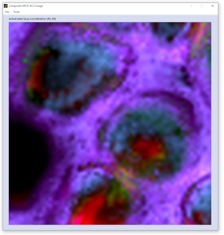
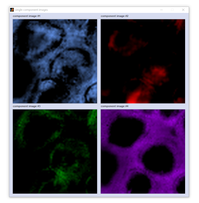
composite i... (composite image): creates a so-called composite image, which is basically a superposition of the individual
component images. In the implementation of CytoSpec ver. 2.00.07 it is also possible to visualize individual components
and to add / remove component representations from the composite image. Please refer to the options 'plot single
components' and 'exclude components' available from the 'Tools' menu bar of the figure 'composite MCR-ALS
image' (see also screenshots below). A detailed description of the functionality is provided in section
composite images of CytoSpec's online documentation.
done: closes the current fit session. Data not stored are lost.
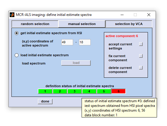
Screenshot of the figure 'MCR-ALS imaging - define initial estimate spectra' with the three
main options 'random selection', 'manual selection' and 'selection by VCA'.
random selection: pressing this button allows defining initial estimate spectra from the HSI on a random basis.
manual selection: permits manual selection of initial estimate spectra directly from the hyperspectral image (HSI) or from reference
spectra by loading them from the file system. Check radio button labeled 'get initial estimate spectrum from HSI' to define a
given pixel spectrum from the HSI, or select 'load initial estimate spectrum' to load a reference component spectrum.
get initial estimate spectrum from HSI: activate this radio button to enable selection of [x,y] pixel spectra from the current
HSI data set as initial estimates. [x,y] coordinates can be entered manually, or by mouse clicks into one of the false color maps
of CytoSpec's main user interface.
load initial estimate spectrum: allows importing an ASCII spectrum as the initial estimate spectrum via a standard file dialog box.
Format of the external ASCII reference spectrum: double column, tab-separated with the first column of frequency / wavenumber
values, second column: intensity/absorbance values.
accept current settings: accepts the currently defined initial estimate spectrum. Clicking onto this button will result in
a green color of the respective component button (see button line 'definition status of initial estimate spectra'). Detailed
information on the status of the respective spectral component is available from the individual tooltips of the buttons
(see screenshot).
fix current component: allows excluding the given initial estimate spectrum from optimization: the given component spectrum
remains unchanged (fixed) during iterations. Pressing this button consecutively toggles between the states fixed / unfixed.
delete current component: removes the currently active spectral component. This is visualized by the red color of the respective
push button in the button row 'definition status of initial estimate spectra'.
Button row definition status of initial estimate spectra: illustrates the definition status of initial estimate spectra.
Assigned components are encoded by green color. Non-assigned initial estimate spectra are shown in red. The tooltip of
each button provides information on the actual settings of the individual initial estimate spectrum. Note that the button
'done' becomes active only in cases where all components are assigned (i.e. the button row is completely colored green).
selection by VCA: initial estimate spectra can be automatically defined by means of
Vertex component analysis (VCA).
Note Pressing buttons 'random selection', 'manual selection'' and 'selection by VCA' overwrites the current
selection of initial estimate spectra.
done: press this button to complete definition of initial estimate spectra. The figure 'MCR-ALS imaging - define initial
estimate spectra' is closed and initial estimate spectra are plotted in the right panel of the figure labeled 'MCR-ALS
imaging''. Initial estimate spectra defined and optimized during earlier sessions are overwritten in this way.
cancel: closes the tool for defining initial estimate spectra and returns to the 'MCR-ALS imaging' dialog window.
Definitions made are not stored, i.e. results from earlier fit sessions are not overwritten.
estimate spectra, or optimized spectra components (left).
main options 'random selection', 'manual selection' and 'selection by VCA'.
load initial estimate spectrum: allows importing an ASCII spectrum as the initial estimate spectrum via a standard file dialog box. Format of the external ASCII reference spectrum: double column, tab-separated with the first column of frequency / wavenumber values, second column: intensity/absorbance values.
accept current settings: accepts the currently defined initial estimate spectrum. Clicking onto this button will result in a green color of the respective component button (see button line 'definition status of initial estimate spectra'). Detailed information on the status of the respective spectral component is available from the individual tooltips of the buttons (see screenshot).
fix current component: allows excluding the given initial estimate spectrum from optimization: the given component spectrum remains unchanged (fixed) during iterations. Pressing this button consecutively toggles between the states fixed / unfixed.
delete current component: removes the currently active spectral component. This is visualized by the red color of the respective push button in the button row 'definition status of initial estimate spectra'.
Button row definition status of initial estimate spectra: illustrates the definition status of initial estimate spectra. Assigned components are encoded by green color. Non-assigned initial estimate spectra are shown in red. The tooltip of each button provides information on the actual settings of the individual initial estimate spectrum. Note that the button 'done' becomes active only in cases where all components are assigned (i.e. the button row is completely colored green).
|
|
Reference to the literature:
[
GENERAL |
FILE |
SPECTRAL PREPROCESSING |
SPATIAL PREPROCESSING |
UNIVARIATE IMAGING |
MULTIVARIATE IMAGING |
TOOLS |
FILE INFO |
GLOSSARY |
CONTACT: info@cytospec.com |
PUBLISHER DETAILS |
PRIVACY POLICY ]
Copyright (c) 2000-2026 CytoSpec. All rights reserved.
FILE INFO |
Copyright (c) 2000-2026 CytoSpec. All rights reserved.